Layer Quant Overview
Quantification of multilayered samples
From measurements on a layered sample at different high voltages, combined with a description of the layered specimen, the Layer Quant software can estimate the thickness and composition of each layer.
The analysis protocol of a multilayered sample is as follows:
1- Standards calibration and definition of quantitative setups at different high voltages, in the same manner as for conventional bulk samples
2- Definition of the points to analyze
3- Association of the analysis points to the different quantitative setups
4- Acquisition of measurements from the layered sample
5- Launching of the Layer Quant software and definition of the multilayer sample (composition and thickness, to a first approximation, for each layer)
6- Data processing with the Layer Quant software
7- Further refinement and display of the final result, yielding composition and thickness of the layers
This software is based on the so-named “X-Film” software developed by Claude MERLET, from the University of Montpellier II France. For details on the calculation method, see: C. Merlet, 1995. A new quantitative procedure for stratified samples in EPMA. Proceed. of Microbeam Analysis, Edited by E. S. Etz, VCH Publishers, p. 203-204.
DEFINITION OF SEVERAL QUANTITATIVE SETUPS
Analysis of a multilayered sample consisting of:
- layer 1 : AuPd, estimated thickness of 8 nm
- substrate : Cu
The data processing for layered sample requires the measurement of the X-rays of the elements at multiple high voltages. The greater the number of beam voltages used, the more accurate the layer thickness and composition estimations will be.
The first step is to acquire calibrations from standards at all voltages to be used in the quantitative setups.
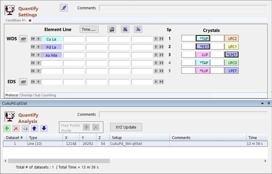
In the example, since the film is relatively thin at 8 nm, low beam voltages are used. Therefore, only lower energy X-ray lines can be excited (Cu Lα, Pd Lα, and Au Mα).
Calibrations are acquired from Cu Lα, Pd Lα, and Au Mα, on pure metal standards, at 5, 7 and 10 kV.
The second step is to define quantitative setups at all beam voltages.
Definition of the analysis setup for Cu Lα, Pd Lα, Au Mα at 5 kV. Analysis setups for 7 and 10 kV are created in a like manner.

The first step is to acquire calibrations from standards at all voltages to be used in the quantitative setups.
Calibrations are acquired from Cu Lα, Pd Lα, and Au Mα, on pure metal standards, at 5, 7 and 10 kV.
Definition of the analysis setup for Cu Lα, Pd Lα, Au Mα at 5 kV. Analysis setups for 7 and 10 kV are created in a like manner.
DEFINITION AND ACQUISITION OF THE POINTS TO ANALYZE
A line of 10 points is defined using the quantitative setup at 5 kV
Use the Duplicate function to create datasets at the same locations as those already defined, using the other analysis setups. It is important that the acquisitions at each setup are made at the same stage positions--the multiple beam voltage data will be combined based on the XYZ values during Layer Quant processing.
Duplication of the existing 10 point line with the setup at 7 kV.
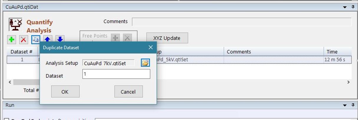
Repeat the Duplicate function until the same set of points, lines or grids are associated with all required setups.
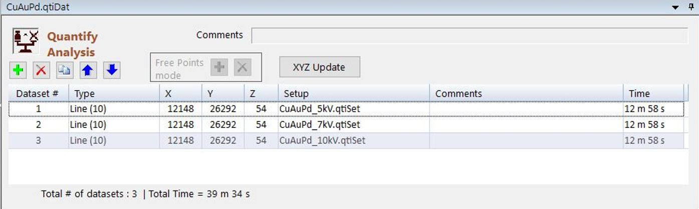
Dataset 1 (a line of 10 points) will be acquired with the 5 kV setup, Dataset 2 (same line) will be acquired with the 7 kV setup, and Dataset 3 (same line) will be acquired with the 10 kV setup.
Finally, acquire all the datasets.
Ongoing results are displayed in the acquisition panel of SxSAB during data acquisition. Do not worry that the totals are not 100%--remember this is not analysis of homogeneous, bulk samples.
When acquisition is complete, open the data file in the SX Results program.
Display of the results
When the acquisition data are first opened in SX-Results, the results appear as they would from homogeneous bulk samples. But because the acquired data are from a layered specimen, the analytical totals will very likely not be 100 wt.%. The data need to be further processed with the dedicated “Layer Quant” software option.
Initial display of the results obtained at 5 kV

Ongoing results are displayed in the acquisition panel of SxSAB during data acquisition. Do not worry that the totals are not 100%--remember this is not analysis of homogeneous, bulk samples.
When acquisition is complete, open the data file in the SX Results program.
MULTI-LAYERED DATA PROCESSING
Display of the results
When the acquisition data are first opened in SX-Results, the results appear as they would from homogeneous bulk samples. But because the acquired data are from a layered specimen, the analytical totals will very likely not be 100 wt.%. The data need to be further processed with the dedicated “Layer Quant” software option.
Initial display of the results obtained at 5 kV
Launching of Layer Quant
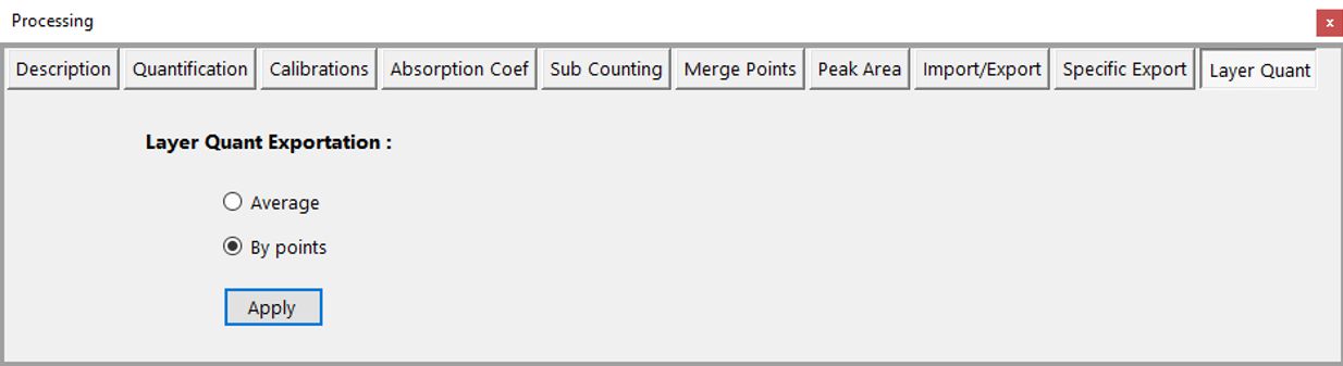
With the data file open in SX-Results, choose the ‘Layer Quant’ tab in the Processing panel. Choose to export ‘By Points’ (that is, each DataSet), or by the ‘Average’ of all points. When the ‘Apply’ button is pressed, a dedicated window opens for Layer Quant processing.
With the data file open in SX-Results, choose the ‘Layer Quant’ tab in the Processing panel. Choose to export ‘By Points’ (that is, each DataSet), or by the ‘Average’ of all points. When the ‘Apply’ button is pressed, a dedicated window opens for Layer Quant processing.
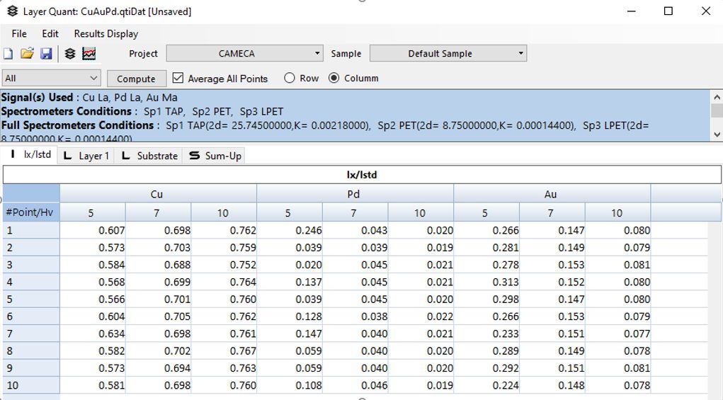
Ix/Istd panel
The first tab of Layer Quant window is the Ix/Istd table. It displays, for each point, the values of Ix/Istd obtained at each high voltage.
Multiple high voltages will be associated to the same point if the X and Y coordinates are identical (Z can be different, if auto-focus is used during the acquisition).
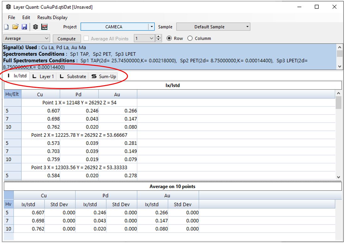
Description of the multi-layered sample
The Layer Quant software requires a sample description to estimate the layers’ composition and thickness. The more information that can be entered into the initial sample description, the more accurate will be the final results.
Click on the sample description button to open the description window or click on the link “To continue, define (or select) a layered sample description”.
Create a new sample description  or use the Load button
  to load an existing description. If creating a new sample description, choose Layered Sample.
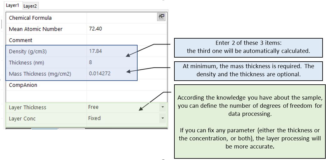
or use the Load button to load an existing description. If creating a new sample description, choose Layered Sample.Note: for the substrate (the final layer), the density, thickness or mass thickness does not need to be entered. It is assumed to be infinitely thick. Only the chemical composition (fixed or variable) is required.
When the description of all layers is complete, click on Save , then click on OK to validate the sample description.
Once the sample description is complete, new tabs are available:
- One tab is defined for each layer, and one for the substrate. In these tabs, all the measurements and calculations relative to one layer are displayed.
- One tab is called Sum-Up, which summarizes the data for all the layers.
At this stage of the process, the data displayed in the table are only based on the description made in the sample description. The Ix/Istd data have not yet been processed and layer thicknesses and compositions have not been calculated.
When the description of all layers is complete, click on Save
Once the sample description is complete, new tabs are available:
- One tab is defined for each layer, and one for the substrate. In these tabs, all the measurements and calculations relative to one layer are displayed.
- One tab is called Sum-Up, which summarizes the data for all the layers.
At this stage of the process, the data displayed in the table are only based on the description made in the sample description. The Ix/Istd data have not yet been processed and layer thicknesses and compositions have not been calculated.
Layer Calculation
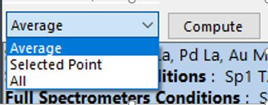
Once the sample description is complete, the Compute button becomes available. There are three different options for the layer calculation, accessed via a drop-down menu. Choose one, then press the Compute button to start the layer calculation.
Once the sample description is complete, the Compute button becomes available. There are three different options for the layer calculation, accessed via a drop-down menu. Choose one, then press the Compute button to start the layer calculation.
Layer calculation on the Average:
- The layer calculation will be made using the average of all the Ix/Istd values present in the Ix/Istd table. The result will be one thickness and one composition per layer, independent of the number of measured points.
Layer calculation from the Selected Point:
- The layer calculation will be made only for the selected point. The number of the selected point is the number displayed in the drop-down list to the left of the Row and Column buttons.
Layer estimation for All:
- A layer calculation will be made for each point for which Ix/Istd has been measured. The result will be a thickness and composition value for each point.
The program adjusts the values of the layer thicknesses and compositions, depending on the degrees of freedom in the sample description, to obtain the best fit between the measured Ix/Istd and the calculated Ix/Istd values.
Results display
Layer estimation for the Average
If the Layer estimation for the Average has been made, check the “Average All Points” box to set the results display to show only the average result.
a) Layer # tabs and Substrate tab
- The layer calculation will be made using the average of all the Ix/Istd values present in the Ix/Istd table. The result will be one thickness and one composition per layer, independent of the number of measured points.
Layer calculation from the Selected Point:
- The layer calculation will be made only for the selected point. The number of the selected point is the number displayed in the drop-down list to the left of the Row and Column buttons.
Layer estimation for All:
- A layer calculation will be made for each point for which Ix/Istd has been measured. The result will be a thickness and composition value for each point.
The program adjusts the values of the layer thicknesses and compositions, depending on the degrees of freedom in the sample description, to obtain the best fit between the measured Ix/Istd and the calculated Ix/Istd values.
Layer estimation for the Average
If the Layer estimation for the Average has been made, check the “Average All Points” box to set the results display to show only the average result.
a) Layer # tabs and Substrate tab
Ix/Istd Calc Calculated ratio between the sample intensity and the standard intensity
Ix/Istd Meas Measured ratio between the sample intensity and the standard intensity
Sigma Mean standard deviation between the experimental values and the calculated values for all the high voltages. Sigma can also be displayed as Relative Standard Deviation (RSD) in the Results Display Options menu.
Ix/Ipure Ratio between the sample intensity and the estimated intensity from a pure element sample
Wt% Weight % concentration
At% Atomic % concentration
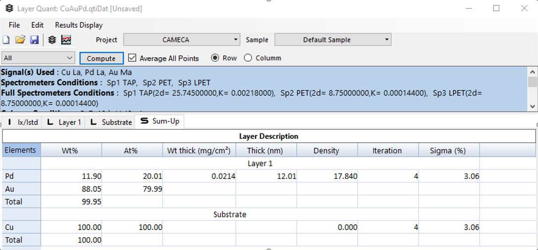
b) Sum-Up tab
Ix/Istd Meas Measured ratio between the sample intensity and the standard intensity
Sigma Mean standard deviation between the experimental values and the calculated values for all the high voltages. Sigma can also be displayed as Relative Standard Deviation (RSD) in the Results Display Options menu.
Ix/Ipure Ratio between the sample intensity and the estimated intensity from a pure element sample
Wt% Weight % concentration
At% Atomic % concentration
b) Sum-Up tab
The Sum-Up table presents the end results of the measurement from the layered sample: thickness and composition of each layer.
Wt% and At% Composition of the layer or substrate (At% is normalized to 100%).
Wt thick Weight thickness in mg/cm² (or select, optionally, µg/cm2 in Results DisplayOptions)
Thick Thickness in nm
Density Density of the layer, in g/cm3
Iteration Number of iterations needed to fit the experimental data to the calculated data
Sigma Mean standard deviation between the experimental values and the calculated values for all the high voltages. Sigma also be displayed as Relative Standard Deviation (RSD) in Results DisplayOptions).
Layer estimation for one or all points
a) Layer # tab and Substrate tab
The panel is divided into two parts:
“Experimental data”: displays the experimental and calculated data for all points and high voltages.
“Average”: displays the average made with all points present in the “Experimental data” table.
Wt% and At% Composition of the layer or substrate (At% is normalized to 100%).
Wt thick Weight thickness in mg/cm² (or select, optionally, µg/cm2 in Results DisplayOptions)
Thick Thickness in nm
Density Density of the layer, in g/cm3
Iteration Number of iterations needed to fit the experimental data to the calculated data
Sigma Mean standard deviation between the experimental values and the calculated values for all the high voltages. Sigma also be displayed as Relative Standard Deviation (RSD) in Results DisplayOptions).
a) Layer # tab and Substrate tab
The panel is divided into two parts:
“Experimental data”: displays the experimental and calculated data for all points and high voltages.
“Average”: displays the average made with all points present in the “Experimental data” table.
b) Sum Up tab
This panel gives the description of the layers for each point

This panel gives the description of the layers for each point
Elements in row or column
For each table, the results can be displayed with the elements in rows (see the examples above) or with the elements in columns.
For each table, the results can be displayed with the elements in rows (see the examples above) or with the elements in columns.
In the Sum-Up panel, if the layers are displayed in column mode, the user can choose to display Wt. Thickness (in mg/cm2 or µg/cm2), Thickness (in nm) or Weight %. In the individual Layer panels, the parameter options are Weight %, Norm Weight %, Atomic% or Oxyde %.


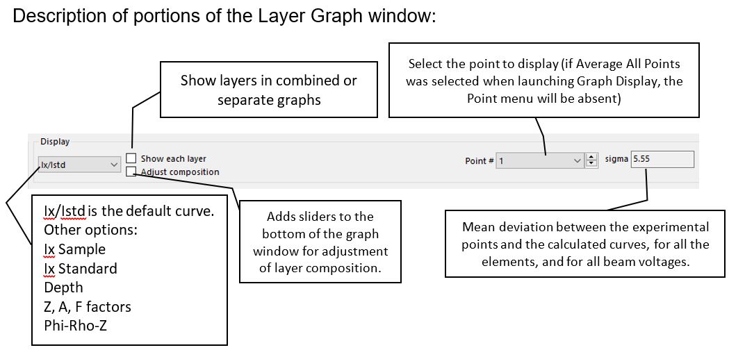
CURVES DISPLAY
After the sample description is loaded, it is possible to simulate and display the curves of Ix/Istd as a function of the beam high voltage.
Click on the curves button:
After the sample description is loaded, it is possible to simulate and display the curves of Ix/Istd as a function of the beam high voltage.
Click on the curves button:
The curves are displayed in a dedicated window named “Layer Graph”.
Description of portions of the Layer Graph window:
Besides Ix/IStd, it is possible to display the following parameters:
Ix Sample: Raw calculated intensity (normalized) as a function of the high voltage for the sample. This takes into account the layers thickness.
Ix Standard: Raw calculated intensity (normalized) as a function of the high voltage for the standard.
Depth: ρzmax = f(HV). Maximum mass thickness (ρzmax) from where the X-rays detected by the counter are emitted.
Z factor: Atomic number correction as a function of the high voltage. This number is relative to the first layer only
A factor: Mass absorption correction as a function of the high voltage
F factor: Fluorescence correction as a function of the high voltage
Phi Rho Z: For one selected high voltage, simulation of the phi (ρz) curves.
Two curves are displayed for each element:
1- The X ray lines generated at a given ρz
2- The X ray line actually counted by the detector, which takes into account (i) the absorption on the X ray line path between the location where it is generated and where it emerges from the sample and (ii) the layers thickness.
Slider controls of thickness and composition:
FILE MENU
Open/ Save/ Save As / Recent
It is possible to save the LayerQuant results as a *.LayQti file with the File/Save function. The LayQti file will save the Ix/Istd values and the sample description. The files can be opened directly in LayerQuant.
The *.LayQti files are saved in the folder : Project/ Sample/Layer Quant/.
Import Quanti Data
Imports a quantitative analysis data file (*.qtiDat file) for processing with Layer Quant.
Import Quanti Setup
Imports a quantitative setup (*.qtiSet) into LayerQuant, which gives an element list to LayerQuant. After defining or importing a layered sample, it is possible to do some graphical modeling of the system with the Curves display.
Select Layered Sample
Function identical to the button, see 4.4 above.
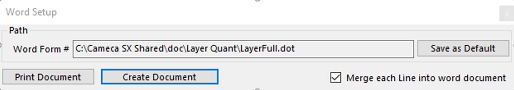
Create Document / Document Setup / Print Document
This function automatically creates an analytical report.
The first time you use this function, select Document Setup to load the template required to make a Word file.
It is possible to save the LayerQuant results as a *.LayQti file with the File/Save function. The LayQti file will save the Ix/Istd values and the sample description. The files can be opened directly in LayerQuant.
The *.LayQti files are saved in the folder : Project/ Sample/Layer Quant/.
Import Quanti Data
Imports a quantitative analysis data file (*.qtiDat file) for processing with Layer Quant.
Import Quanti Setup
Imports a quantitative setup (*.qtiSet) into LayerQuant, which gives an element list to LayerQuant. After defining or importing a layered sample, it is possible to do some graphical modeling of the system with the Curves display.
Select Layered Sample
Function identical to the
button, see 4.4 above. Create Document / Document Setup / Print Document
This function automatically creates an analytical report.
The first time you use this function, select Document Setup to load the template required to make a Word file.
Then you can use Create Document.
The Word document will contain:
The Header of the Layer Quant window
The experimental data (Ix/Istd)
The sum-up tab
The data will have the same format as those displayed in the Layer Quant window: Column or Row
The Layer Graph window (experimental dots and calculated curves)
The Word document will contain:
The Header of the Layer Quant window
The experimental data (Ix/Istd)
The sum-up tab
The data will have the same format as those displayed in the Layer Quant window: Column or Row
The Layer Graph window (experimental dots and calculated curves)
Exit
Exits the LayerQuant program.
EDIT MENU
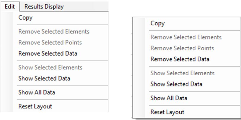
Exits the LayerQuant program.
EDIT MENU
The functions in the Edit menu are also available with a RMB click in the data table:
Copy
Copies data in the current table to the clipboard. The data can then be pasted into documents of other application programs, such as Word or Excel.
Remove Selected Elements / Selected Points / Selected Data
It is possible to exclude unwanted measurement data from the Layer Quant calculations by manipulation of the Ix/Istd table. This might be done to remove outlier data. The data are not permanently removed from the datafile--they are only suppressed from the calculations and can be restored at any time. It is possible to exclude data by element, by beam voltage, by point, or by individual measurement. Selection of multiple cells is possible by using shift-LMB (for continuous selection) or ctrl-LMB for discontinuous selection).
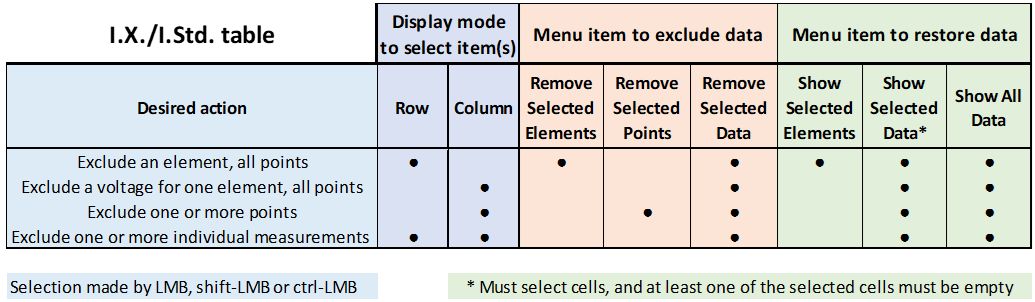
The following chart shows possible data exclusions, along with the required Ix/Istd display mode and menu commands:
Copies data in the current table to the clipboard. The data can then be pasted into documents of other application programs, such as Word or Excel.
Remove Selected Elements / Selected Points / Selected Data
It is possible to exclude unwanted measurement data from the Layer Quant calculations by manipulation of the Ix/Istd table. This might be done to remove outlier data. The data are not permanently removed from the datafile--they are only suppressed from the calculations and can be restored at any time. It is possible to exclude data by element, by beam voltage, by point, or by individual measurement. Selection of multiple cells is possible by using shift-LMB (for continuous selection) or ctrl-LMB for discontinuous selection).
The following chart shows possible data exclusions, along with the required Ix/Istd display mode and menu commands:
Some examples:
Excluding an element from all points and voltages in the Layer Quant calculations: Row Display, click on the element heading, then choose Remove Selected Element.


Excluding an element from all points and voltages in the Layer Quant calculations: Row Display, click on the element heading, then choose Remove Selected Element.
Excluding several points: Column Display, use ctrl-LMB to select individual points, then choose Remove Selected Points.
Excluding individual measurements: Row or Column display, use ctrl-LMB to select measurements, then choose Remove Selected Data:
Show Selected Elements / Selected Data
The ‘Show Selected Elements’ and ‘Show Selected Data’ commands restore previously excluded data to the I.X./I.Std. table. These commands are useful if a full restore is not desired.
Example:
Three measurements (Points 1, 2, and 4, at 7 kV) have been excluded for Pd and it is desired to restore only one of the data points (for Point 1). Select the cell (Point 1, Pd at 7 kV), then choose the menu item ‘Show Selected Data’.
The measurement has been restored:
Show All Data
Use ‘Show All Data’ to restore all data previously, as they were in the original file.
Reset Layout
Restores the display layout to the default layout, for example, if data columns have been resized or hidden.
RESULTS DISPLAY
Use ‘Show All Data’ to restore all data previously, as they were in the original file.
Reset Layout
Restores the display layout to the default layout, for example, if data columns have been resized or hidden.
RESULTS DISPLAY
Header content
Select the items to display in the header part of the main window.
Select the items to display in the header part of the main window.
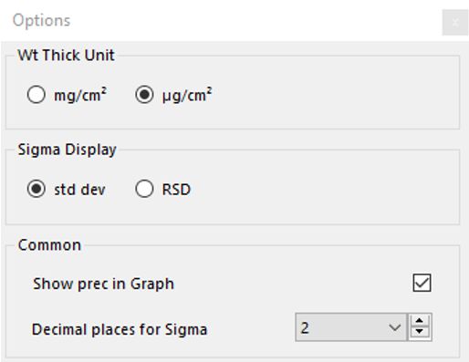
Options
The Options menu controls some displays used in the program.
Weight Thickness Unit (mg/cm2 or µg/cm2)
Sigma Display (standard deviation or Relative Standard Deviation)
Common
Show precision in graph (shows Sigma by each element on curves graph)
Decimal places for Sigma
Note: the Curves display may need to be closed and reopened to see the effect of any parameter change in the Options window.
Export selected / all points to Excel / Excel setup
This function allows data export to Excel, and at the same time makes a graph of the exported data. For this reason, the exported data should be in column mode: the X axis of the graph will be the point reference; the Y axis will be the item selected for the column display mode.
Display the data in Column display
In Excel setup, define the Excel template to be used to export the data
Select with LMB the points to export and select Export selected points To Excel to export only some points or select Export all points To Excel to export all points.
The data are sent to Excel.

The data are sent to Excel.
Contact

Our support team is ready to help you
FAQ

Answers to some common questions from SX users
Troubleshooting

Quickly search for solutions to instrument issues