SX-Control – WDS & Spectro

Overview

This section gathers all the functions and information dedicated to the Wavelenght Dispersive Spectroscopy (WDS) settings and analysis parameters. 

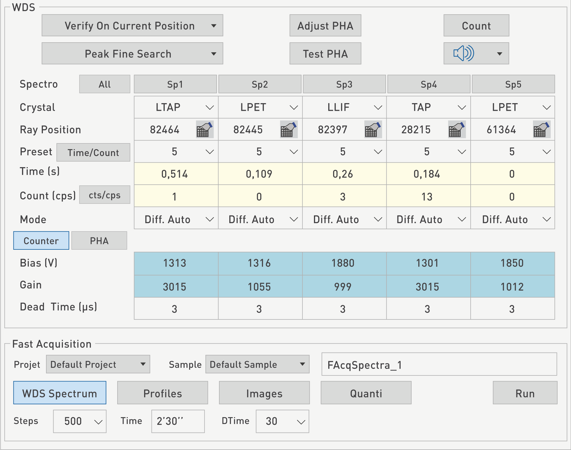
Spectrometer selection 

In the ‘Spectro’ frame, users have the possibility to select up to five spectrometers (Sp1 to Sp5), depending on the instrument configuration. All spectrometers can be selected at once by clicking on ‘All’ button. Selected spectrometers are on a blue background while unselected ones have a grey background.

Note: Better statistics are generally achieved with more spectrometers than less, however, this is only valid when all spectrometers are gathering the same type of data or counts. An EPMA instrument is usually equipped with various crystal types to be able to probe almost all the elements of the periodic table (from Lithium to Uranium), since a single crystal can only cover a limited range of elements and X-ray lines. Therefore, each spectrometer, from SP1 to SP5, potentially has between one and four crystals, depending on the users’ needs and on the type of crystals. The maximum number of crystals a spectrometer could accommodate is two for the large crystal types, and four for the small or regular crystal types. Large crystals have a larger area and provide higher counting rates than normal crystals.

The desired crystal can be selected by the Crystal drop-down menu below each spectrometer reference. Small crystals are indicated by a 3-letter designation. The most common are LiF, TAP, PET, PC1, PC2, PCN. Large crystals are indicated by a 4-letter designation such as LLiF, LTAP, LPET, etc. In the nomenclature adopted by CAMECA, the extra ‘L’ letter prior to the crystal name stands for ‘Large’.

The typical configuration for a WDS Survey scan on a totally unknown specimen is PC2, TAP, PET and LiF. This configuration enables the exploration of almost the entire periodic table (from B to U).

Spectrometer modes

Now that the counting sequence is understood, it will be useful to consider the counting Modes available, as the PHA (Pulse Heigh Analyse) operates in two distinct modes, respectively the Integral mode, and the Differential mode.

In Integral mode, the Baseline is set by default (with a Zener diode) at 560 mV and the window width at 10 V. The width of the distribution is usually defined at 50% of the maximum or Full Width Half Maximum (FWHM). All pulses within this window are counted. This is the most commonly used mode.

The total number of counts includes the true counts from the selected diffraction line, the background counts (Bremsstrahlung, matrix effect, specular reflection on the crystal), some counts from photons with multiple orders-of-magnitude higher energy which could be present (sample dependent) knowing that nθ = 2d sinθ, with n > 1, and any noise generated by the physics and electronics of the instrument.

The Differential working mode might be necessary if the following case occurs. It may happen that at a certain spectrometer position and with a specific crystal, one collects a first diffraction order line of an element and a multiple-order reflection line of another element. This could be the case for instance between O K 1 and Al K 3 (3rd diffraction order of Al K line) on a PC2 crystal. Both photons are seen at the same wavelength, but as their energies are different, the collected pulses have different heights. By setting the Baseline and the Window width to the appropriate values, one will be able to suppress, or at least minimize the influence of the higher order reflection line. Therefore, with this Differential counting mode, only the pulses corresponding to the first diffraction order line will be taken into consideration. A schematic describing the terms involved in setting up the parameters for Pulse Height Analyzer (PHA)distribution is shown below.

If at a diffraction position (sine θ), a crystal indicates the energy position E0 for the maximum energy distribution, then the corresponding FWHM value is W0.

So the key point of the differential mode is to skillfully choose the right limits to achieve this distinction between elements of various diffraction order lines.

Note: this mode cannot suppress interferences between two elements if they are both at the first diffraction order line.

In the Differential Automatic Mode, Baseline and Window width values are automatically computed with respect to the theoretical selected energy line. The key point is to make sure the PHA parameters are properly set prior to using this Automatic mode (see PHA paragraph below in this section to ensure PHA is set-up correctly).

Spectrometer alignement

As stated above, each crystal type will allow only a certain range of wavelengths to diffract. Therefore, in order to properly position the crystal to gather the signal from the diffracting lines, the Ray Position (based on Bragg’s law) must be found. An X-ray line position is either entered by typing a number corresponding to the (10000 x Sin θ) value into PeakSight, by typing the element name as it reported on the periodic table, or automatically found by clicking on the periodic table.

A number of steps relative to a position already reached, either to the right of that position (r+) or to the left of it (r-) can also be type.

Note: Users should also realize that the mechanical swapping from one crystal to another will induce a mechanical mismatch or displacement on the order of a few µm. This is sufficiently large to prevent the crystal from being at the exact diffracting position required for the X-ray lines to provide the best intensity signals. Therefore, anytime a mechanical swap or crystal rotation is made, a verification operation routine called Peak Verify must be performed.

One can use a position already stored in the software, knowing that each crystal type has some characteristic strong signals emitted for specific X-ray lines. One can also proceed to Verify on a non-stored position, but users would have to use a Current Position which would then be set.

The Verify routine is equivalent to an energy calibration of the WDS spectrometers. It performs a position calibration of the WDS spectrometers using a known specimen with known elements and well-defined position lines.

When the Verify routine is activated, each selected WDS spectrometers moves to the theoretical position of a well-defined line. A Peak Search routine is performed around this theoretical position to measure the observed position of this line. The program computes the shift in position between the observed position and the theoretical one. The entire spectrometer positions are then shifted from the computed value. The shift can be positive or negative in Sin θ  units.

Note: The ‘Verify’ and the ‘Peak Search’ routines will only be accurate and trustworthy if the beam is very well focused optically on the sample surface. Therefore, the Autofocus step is strongly recommended.

The red color in the Ray Position window simply indicates that the current crystal positioning has not been verified and aligned yet for that spectrometer.

Periodic table

On the periodic table, the spectrometer number (SP), the associated crystal type (Xtal) and the accelerating voltage (HV kV) are readily visible. 

Based on these 3 parameters, only a limited list of elements will be eligible for selection, and users must specify the Reflection Order line (1, 2, 3, etc.), as well as the X-ray line (K, L, M, K, L, M, etc.). The color coding in the periodic table uses Red for the K line series, Blue for the L line series, and Purple for the M line series. By default, the most intense line of a series is highlighted. They are:

- K line for the K series,

- L line for the L series,
- M line for the M series.

A selected spectrometer moves to the position corresponding to the chosen line. The line symbol is then printed in the Ray Position field and the Periodic Table closes automatically after a line selection.

The spectrometer offset measured during the Verification routine is taken into account. To ensure that the spectrometer is exactly on top of a selected peak it is recommended to perform a Peak Search.

Peak Search

A drop-down menu is available under the default ‘Peak Fine Search’ function. It allows a user to perform the detection of the peak position where the intensity will be the highest within the WDS scanning window. This search window can be large, in which case a ‘Peak Wide Search’ is performed, or this window can be narrow and a ‘Peak Fine Search’ is performed. The Wide, then Fine Search is also possible to ensure the WDS scanning window has taken into account the most intense peak in the area.

A user can also look for a specific X-ray line by using ‘User Defined Wide’ and ‘User Defined Fine Search’ options.

The result of the Peak Search is displayed in the multipurpose panel (Wds Curve) of the SX-Control module under the ‘WDS Curves’ tab.

Time and Count setting

Users have the ability to set up a pulse counting time for the measurement on each individual spectrometer by using the Time Preset (s) drop-down menu, or by typing a desired value. Then, once a measurement has started by clicking on ‘Count’ button, the value in the Time (s) window will evolve until it reaches the value defined in the Time Preset (s) window and the counting sequence is finished. In parallel, a number of Counts (cts) or Counts per Second (cps) will be displayed. These two values, cts and cps, are only visible one at a time, and can be interchanged or toggled by a left click on ‘cts/cps’.

Bias and Gain

When an electron beam irradiates a small area of the sample, the X-ray induced emission that is selectively diffracted with respect to the wavelength due to an X-ray monochromator. The diffracted signal enters the chamber of a gas flow-based detector which is maintained under a high voltage bias; this device converts the detected photons into electrical pulses. These pulses are then sent to a counting electronic chain involving a pre-amplifier (to transmit the signal without affecting the detector), a pulse amplifier (to allow analysis of the signal), a pulse discriminator (PHA, to sort the pulse energies), and an integrator (to count the pulses). The number of counted pulses N depends on the number of collected X-rays.

The Bias applied on the anode has to be adjusted to give a pulse whose height is proportional to the photon energy. This regime is called the region of proportionality. 

Typical Gain and Bias values are reported in the table below.

Dead Time

The counter Dead Time is the time during which the counter is called «blind». When a pulse has been collected on the Anode wire, the associated electronics requires a certain time before being able to count the next pulse. This time is called the Dead Time. During instrument construction it is adjusted in the electronic circuit to 3 micro seconds and it is usually not necessary to change it.

PHA

The Pulse Height Analyzer (PHA) is a circuit that sets a superior threshold and an inferior threshold. Only the pulses whose height lie within the window defined by the Baseline (inferior threshold) and the Window width (superior threshold) are counted. All the pulses whose height is below the Base Line and above the Window are rejected and not counted.

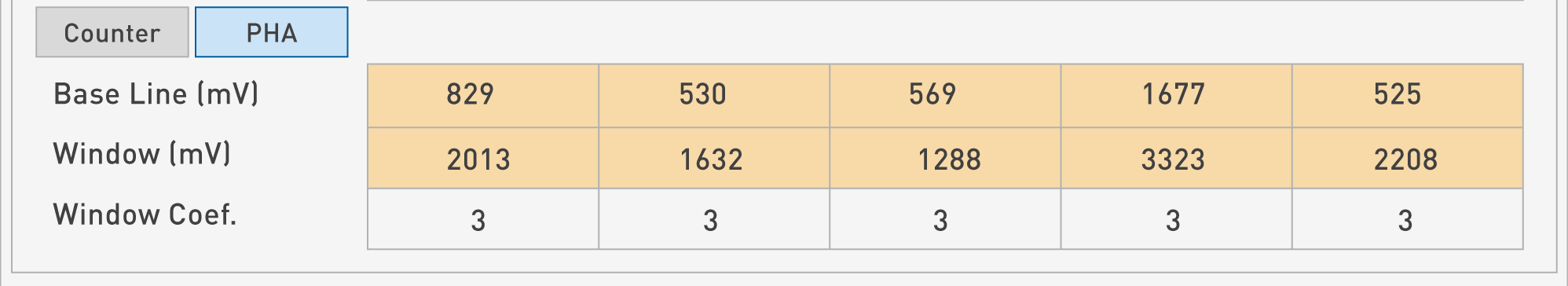
Althrough the Test PHA and Adjust PHA functions are located in the window we have defined as WDS #1 (WDS frame), the corresponding values for Bias, Gain and Dead Time are located in the WDS #2 (Spectro table).

The ‘Test PHA’ function records the pulse distribution in the current spectrometer position when activated by a left click. The test is performed with the actual bias and gain values on the selected spectrometers. In order to record a pulse height distribution, it is recommended to move the stage to a known specimen and select a spectrometer as well as the desired X-ray diffraction line. If necessary, one could use the Peak Fine Search function to locate the chosen line. 

Upon clicking on the Test PHA, a graphic window is automatically generated and displays the energy distributions of the selected spectrometers at the end of the acquisition for each spectrometer.

Regarding the three parameters in WDS #3, the Bias is simply the counter anode wire high voltage value (V), the Gain corresponds to the PHA board gain value (dimensionless) and the Dead Time of the PHA board is expressed in µs.

In practice, after using the Test PHA routine, it’s quite easy to assess the quality of the pulse distribution in terms of its positioning. If the Test PHA is satisfactory as shown below (Fig. b), then no adjustment is necessary. However, if the outcome of the Test PHA is as shown on Fig. a, then a left click on ‘Adjust PHA’ is surely required to properly center the energy distribution (abscissa in V).

In the current spectrometer position, the ‘Adjust PHA’ routine carefully pairs the gain of the electronic amplifier and the voltage applied on the anode (Bias) to set the counter in the proportional mode. The routine keeps iterating until the pulse distribution is well positioned. 

WDS Curves

All the WDS curves showing the peaks and their related energy distributions are readily visible in the ‘Multipurpose panel’ (Wds Curve) of the SX-Control menu, under the tab ‘WDS Curves’. The number of graphs displaying diffraction lines or energy distributions will be linked to the number of spectrometers selected for the experiment.

Users use the ‘Save Peak’ and ‘Save Distribution’ according to the ‘Spectrum’ or ‘PHA’ tab respectively. The recording format is in ASCII. 

Saved data are accessible at the following folders:

Spectrum path:

 C:\CamecaSX Shared\Logbook\Spectrum 

PHA path:

 C:\CamecaSX Shared\Logbook\PHA 

Note: Filenames will contain embedded information such as spectrometer number, crystal type, as well as the date and time stamps at the time of file creation.

Buzzer

The drop-down menu associated to the speaker icon allows to enable a buzzer that transform count number on the detector into mono-frequency sound. The buzzer volume can also be set through a discrete noise level by increment of 25% (0, 25, 50, 75 and 100). This function is useful when a user is focusing on other tasks while the measurement is being acquired.