SX-Result WDS

Overview

WDS Spectra are one of the most efficient ways to explore a sample’s chemical composition. The resulting spectrum has an excellent spectral resolution and contains thousands of single measurements. This database can be used to identify the occurrence of chemical elements within a given sample and also get semi-quantitative analysis with or without calibration.

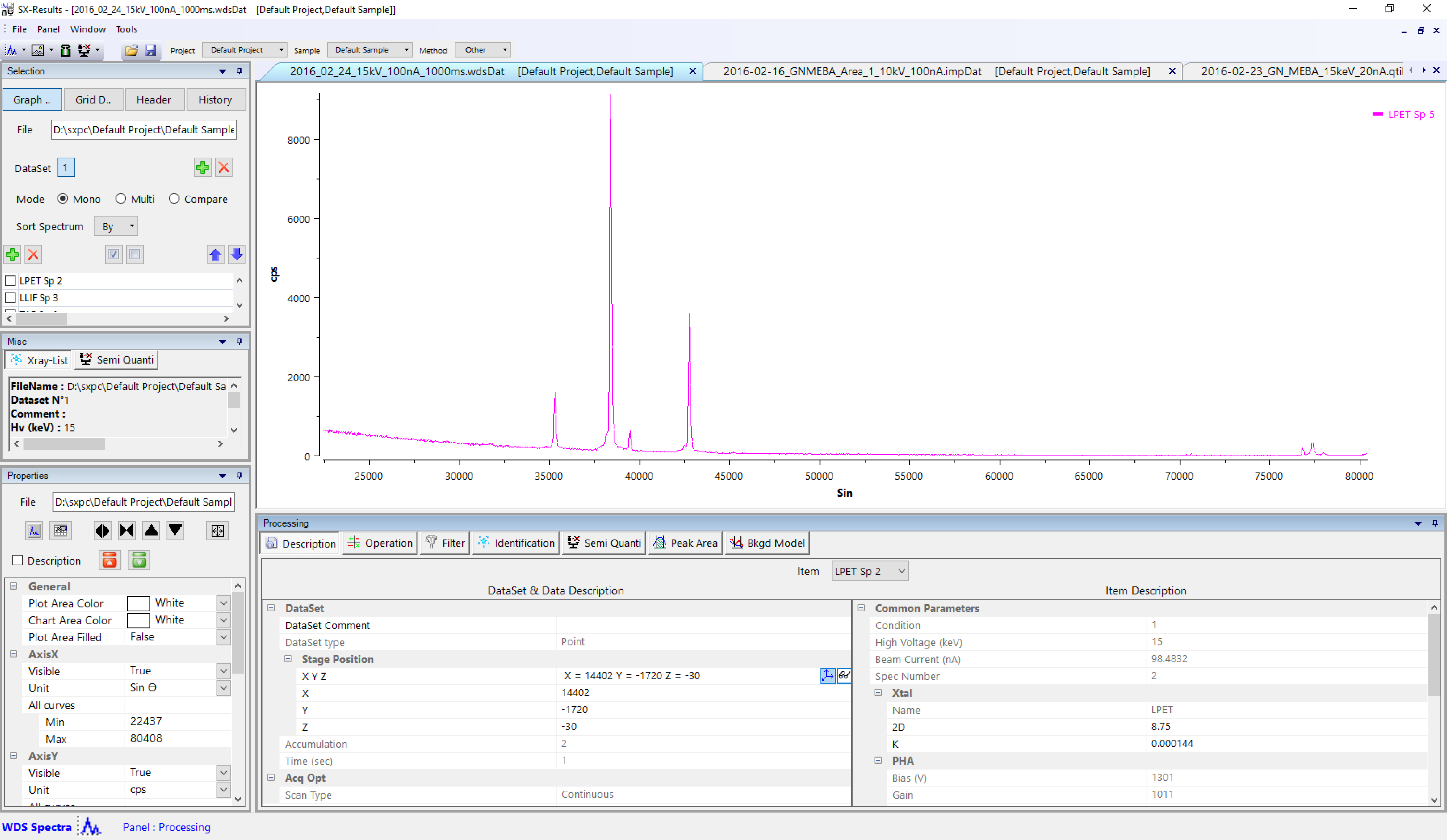
When a user opens a WDS file, spectra (up to five) are displayed in the result viewer, under a specific tab (highlighted in blue). Functions of the Processing panel are specifically dedicated to spectrum analysis, as well as the ‘Selection’, ‘Misc’ and ‘Properties’ panels on the left side of the SX-Results window.

‘Selection’, ‘Misc’ and ‘Properties’ panels

Selection panel

This panel organizes and allows selection of all the data displayed inside the data viewer. For each file, users can display a graphic view (‘Graph Data’, e.g., spectrum, images), its corresponding data grid (‘Grid Data’), its related header (‘Header’) that contains all the options and settings of a given analysis, and a log (‘History’) that registers all the modifications that affected the file during the SX-Results processing, by clicking on the related buttons. ‘Grid Data’ allows the user to modify spectra, profiles or images. All the modification are registered in the ‘History’ log.

File

Displays the current file name and path.

DataSet

Users can also select, add or delete dataset from the original data file using the DataSet functions.

Mode

Allows spectra to be display all on the same graph (‘Mono’), one graph for each spectra (‘Multi’) or two or more spectra (‘Compare’).

Sort Spectrum

Sorts the spectra displayed in the Result viewer according their wavelength (decreasing or increasing).

Spectrometer list

Gives a list of the available spectrometers subject to the conditions of a given analysis. Users can easily select which spectrum they want to display as well as import (‘+’) or delete (‘X’) a spectrum, or rearrange the the list.

Misc panel

This panel contains some basic information like the ‘Xray-List’ and ‘Semi Quanti’. The latter is the result of the ‘Semi Quanti’ processing described below.

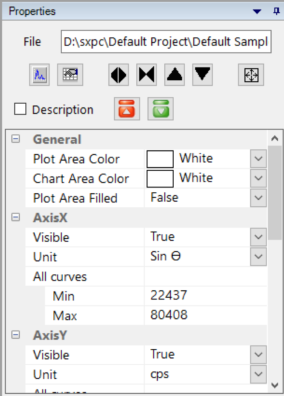
Properties panel

This panel is dedicated to spectrum analysis and display. 

File

Displays the current file name and path.

KLM Lines

The ‘Show/Hide KLM Lines’ button together with the ‘Periodic Table’ button gives the user an easy way to recognize chemical elements directly on spectrum. The ‘Periodic Table’ simplifies the element detection by selecting only the elements of interest. Four visualizations option are available through the ‘Show/Hide KLM Lines’ as follow:

- 1 click: display only black vertical lines for each detected peak that corresponds to a known chemical element.

- 2 clicks: display only the name of the predicted element on each detected peak that corresponds to a known chemical element.

- 3 clicks: Same as for 2 clicks, the element name is preceded by the ray name (Ka, Kb, La, Lb, etc.)

- 4 clicks: display all the above information together.

Graph scale

The four buttons with black arrows together with the arrow/square button allows the user to change the  graph scale horizontally (expand  or compress ) or vertically (expand  or compress ), or reset the scale.

Option List

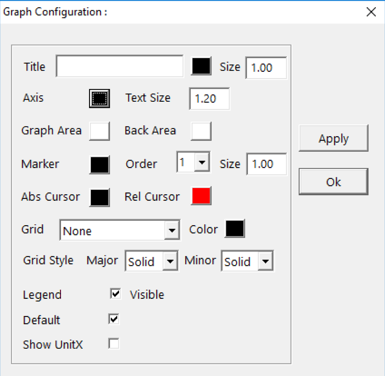
The list gathers all the available graph options for ‘AxisX’, ‘AxisY’ and ‘Items’. Colors, shapes and scales can be set through their dedicated options.

Some other options are available by double-clicking on graphs or curves.

Processing panel

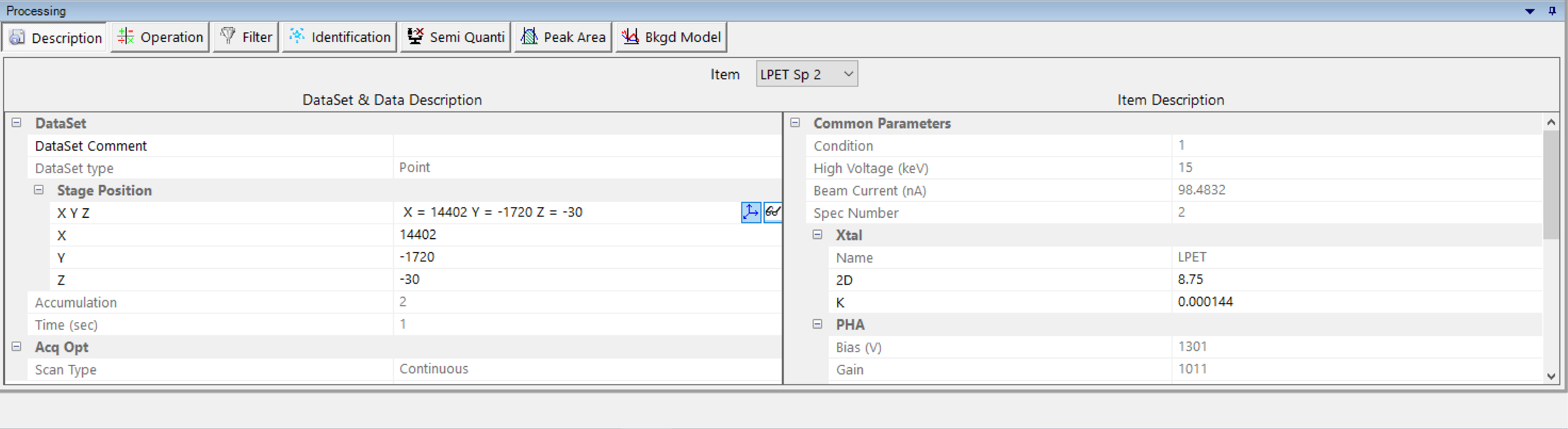
Tools for spectrum processing can be accessed through the ‘Processing’ panel.

Description

Gathers all the settings and options defined together with the WDS setting file through the SX-SAB – Settings. The drop-down list allows the user to select the desired spectrum through the corresponding spectrometer. Most of the information is read-only but some can be modified like ‘Stage Position’, ‘Xtal’ or ‘Starting Position’.

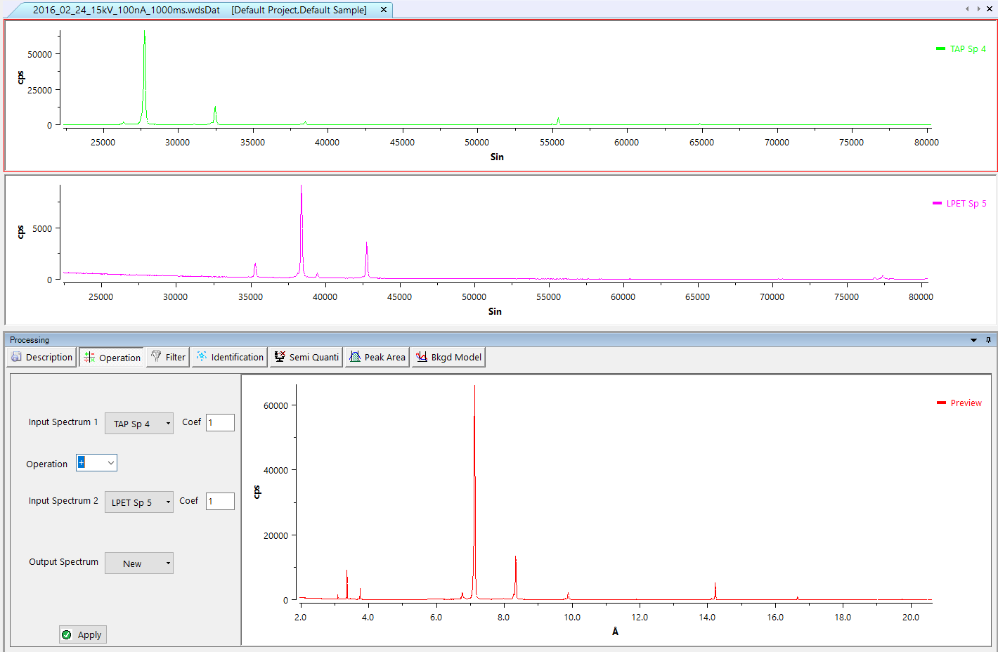
Operation

Allows users to sum, subtract, multiply or divide two selected spectra from the original WDS data file. The ‘Output Spectrum’ drop-down list indicates the place where the calculated spectrum will be drawn. The apply button displays the result of the operation to the current dataset.

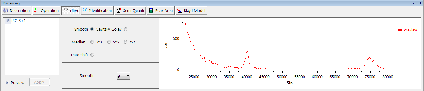
Filter

This tool applies filters on selected spectrum. The preview checkbox displays, in real-time, the filtered spectrum inside the filter tool. Default filters are the following:

Smooth

Smooth the curve, merging close points.

Savitzky-Golay

The Savitzky–Golay filter increases the signal-to-noise ratio without greatly distorting the signal to smooth the data. This is achieved, in a process known as convolution, by fitting successive sub-sets of adjacent data points with a low-degree polynomial by the method of linear least squares.

Median

Merge points in a given area: ‘3x3’, ‘5x5’ or ‘7x7’.

Data Shift

Shift the whole data to the right (positive Sin θ) or to the left (negative Sin θ). The shift value is defined as Sin θ. 

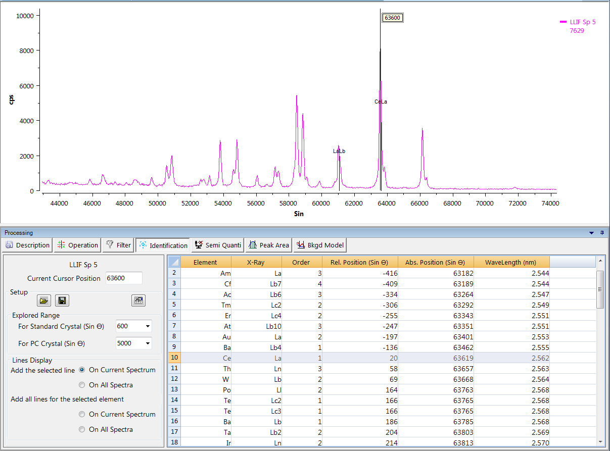
Identification

An easy-to-use tool to identify a chemical element occurrence from the selected spectra. Users set the cursor position (Sin θ), or the explored range according to the chosen spectrometer (Standard crystal or PC crystal) and the line display. The ‘Periodic Table’ icon allows the user to restrict the elements that can be detected.

Semi Quanti

Since PeakSight 6.2, we propose a new WDS Semi-Quantitative software that allows extraction of the composition of any sample from WDS spectra, both qualitatively (using a new element auto-identification routine) and quantitatively (using either standardless or measured calibration).

The Semi-Quantitative program will be efficient if WDS spectra are acquired under good conditions. Typically, the following conditions are required:

- All crystals used in the WDS spectra have to be verified before the acquisition is launched.

- The set of crystals must be chosen so that all expected elements have at least one major line (Kα, Lα or Mα) ;

- Good counting statistics are also required, which is generally achieved with the following conditions: 20 kV, 100 nA, 200 ms dwell time and 1000 channels.

- We recommend to make the acquisition with PHA in Automatic mode in order to avoid multiple identification due to second order or more X-ray lines, and in order to efficiently use the calculated standards.

Provided the above conditions are met, the Semi-Quantitative program will give weight% results with a typical precision of +/-5% for K lines elements and +/-10% for L or M lines elements.

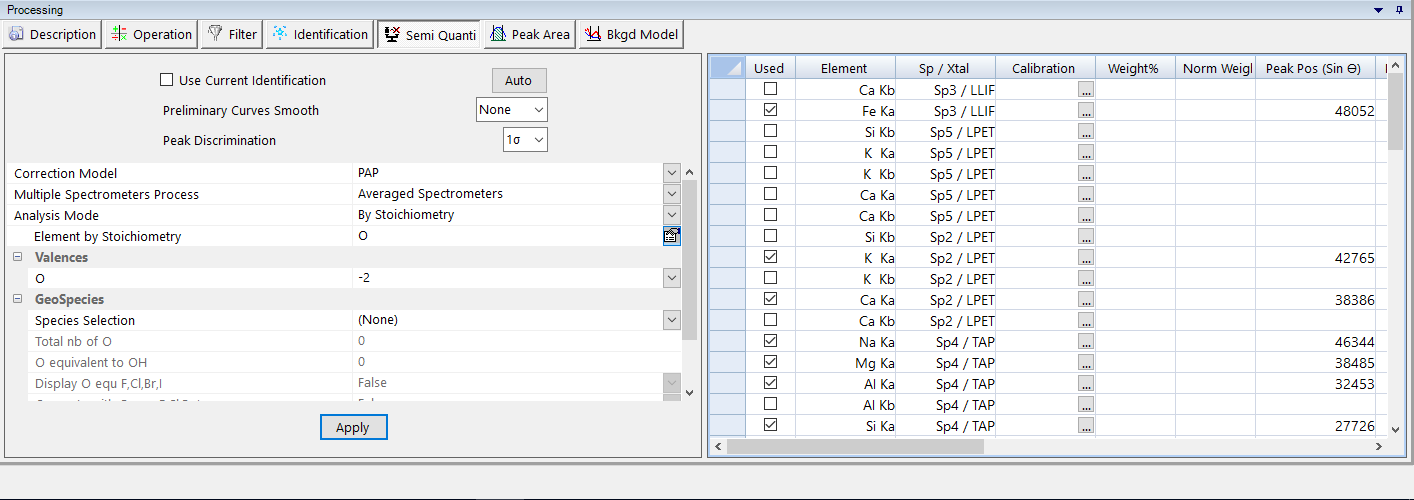
The Semi-Quanti process requires identification of the different peaks. Current identifications defined from the ‘Properties panel’ is used by default, but users can also choose an automatic identification by unchecking the ‘Use Current Identification’ and clicking on the ‘Auto’ button. Then, the list of the elements identified for the Semi-Quanti analysis is displayed on the right side of the ‘Semi-Quanti’ sub-panel. Selected elements are specified by checking the ‘Used’ checkbox.

Smoothing options are also available but not required to prevent artifacts on low intensity peaks. in addition, the process needs a ‘Peak Discrimination’ routine (1 σ or 2 σ).

Before running the Semi-Quanti process, users have to select the ‘Correction Model’, the ‘Multiple Spectrometers Process’ and the ‘Analysis Mode’, and to attach calibration file to the selected elements of the list.

If a calibration file has not been selected for some elements, a theoretical calibration file is generated according to the ‘Efficiency Acquisition’ data.
The acquisition of the efficiency files is automated with the program SemiQtAcquisition9.exe (in C:\Program Files\CamecaSX\bin folder).

One click on the ‘Apply’ button displays the quantification on the ‘Semi Quanti’ tab of the ‘Misc’ panel.

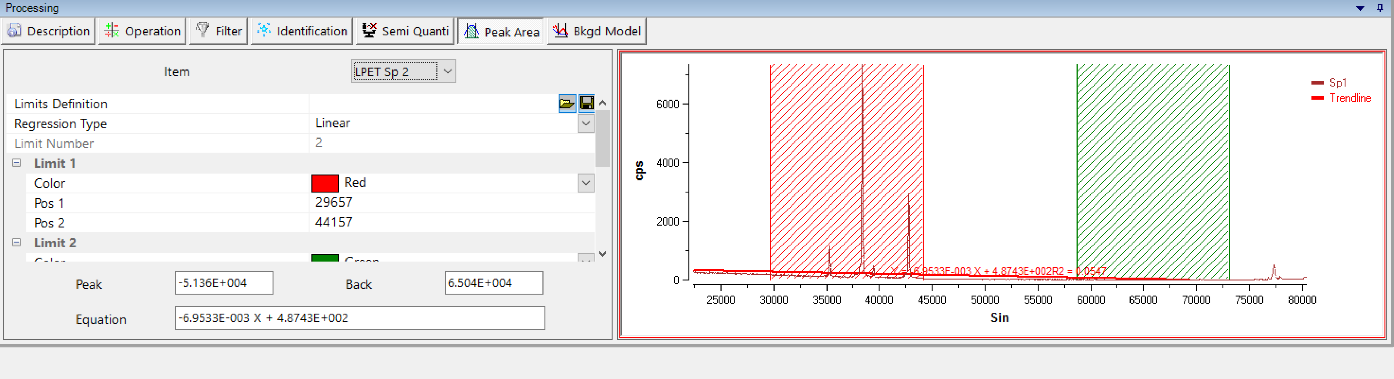
Peak Area

Element calibration can be run according to two methods: by peak intensity or by peak area measurement. The latter requires a definition of the surface which must be considered for further calculation. The ‘Peak Area’ process allows the definition of a reference geometry for a given peak from any selected spectrum.

Combining exclusion areas (by default red and green hashing's) and regression line (linear, polynomial, exponential or power) for the background, users can easily obtain the reference peak area and then save it as a ‘Limit Definition’ for the calibration (see the SX-SAB Settings for further information about the calibration process).

Previously saved ‘Limit Definition’ can also be loaded, modified and saved.

Bkgd Model

Similar to the ‘Peak Area’ process, the ‘Bkgd Model’ process (for Background Model) models the expected background shape under analytical conditions for each spectra. This function is useful when the background is complex and uncorrectable with a simple linear regression.

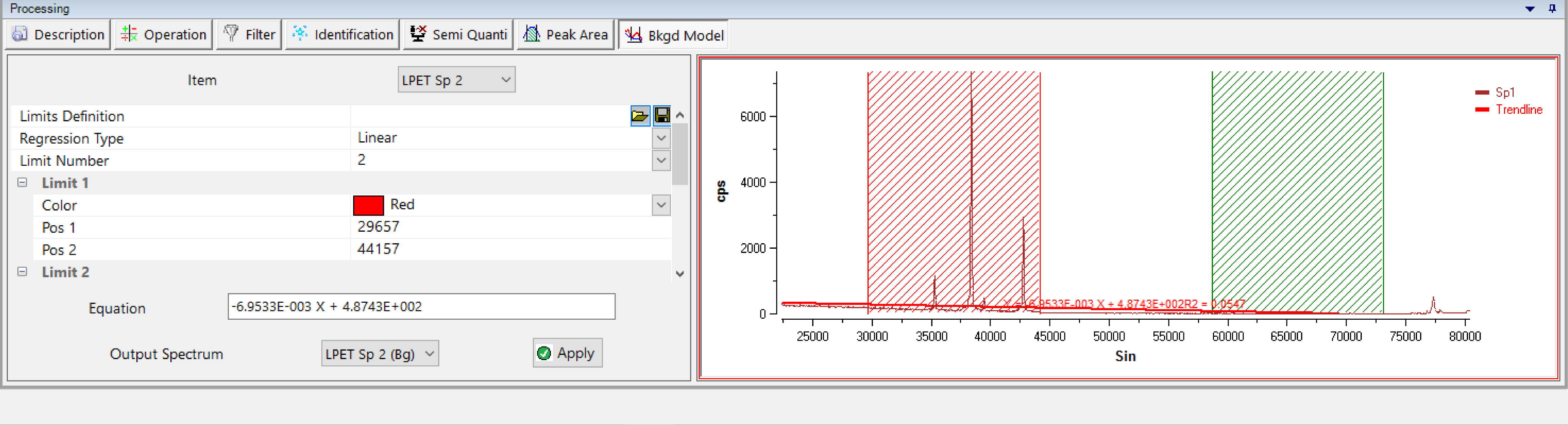
Combining exclusion areas (by default red and green hashing's) and regression line (linear, polynomial, exponential or power) for the background, the calculated model can be saved or applied to the output spectrum (not necessary the reference spectra).

Previously saved ‘Limit Definition’ can also be loaded, modified and saved.