SX-SAB – Analysis

Overview

The analysis mode of the SX-SAB gives the users the ability to acquire data according the settings defined previously. WDS Spectra, Images & Profiles, Calibrate and Analysis are described below. The Tutorial section (link) offer more information about step-by-step procedures for some practical cases. The general window organization is the same as in the of SX-SAB Settings mode. The properties panel is dedicated to DataSet #, Dataset # Options, and Common Options.

WDS Spectra Analysis

Users can create an Analysis file in the WDS scan mode by clicking on the ‘New File’ icon after the combined selection of the WDS icon and the ‘Analysis’ mode button enabled on the shortcut icon bar or use the File  New  Analysis  WDS Spectra string or directly edit the properties of the panels below the icon menu. Users can also click on the ‘Acquire Now’ button available through the WDS Spectra Setting panel.

Any WDS Analysis file will be easily recognized by its « .wdsDat » extension. Therefore, once defined, this name will also be associated to the Properties and the WDS Spectra Analysis panels, as shown above.

On the ‘Properties’ panel, the first step in the definition of a WDS ‘Analysis Setup’ file would be to assign a specific stored WDS Setup file to dataset. The folder icon under the DataSet part, allows users to choose from a list of « .wdsSet » files.

The location always starts with a point or (X, Y, Z) coordinates by default. One click on the ‘glasses’ icon updates the XYZ values to the current stage position. If that location is satisfactory, then it could be assigned to the DataSet by clicking on the coordinates icon.

Still in the Stage sub-panel, users can define the number of points measured (‘#points’, the number of cycles (‘# Accumul.’) and the ‘Dwell Time (ms)’ per channel.

DataSet# Options

Under the ‘DataSet# Options’ tab, if the ‘Continuous’ option is validated ([True]), it means that the selected spectrometer is moving at a continuous speed (Sin θ per minute) during the entire spectrum scan. Intensities are recorded and stored every ‘Dwell Time’. If the Continuous option is set to [False], the spectrometer moves in a step-by-step mode, which is more time consuming than the Continuous mode, but allows very long counting times to be performed since the counting starts during the programmed Dwell Time. 

The Beam Setup could be loaded [Once] per DataSet or at [Every Point] defined in the DataSet. Users could also choose to have the actual [Current] beam setup as default when running the WDS Analysis.

Common Options

Within the ‘Common Options’ tab, some options are applied independently of all the datasets. They consist in checking the physical positioning of the spectrometers either after flipping from one crystal to another on the same spectrometer, or just before starting an analysis as a safe procedure. A ‘Wait Time (s)’ could be added in order to enable the beam to be stable on same materials types for example. A recurrent option could call to ‘Load Setup’ at a chosen frequency.

With SX5-Tactis it’s possible to acquire EDS spectra on each pixel of an image selecting ‘True’ on the EDS Hypermap option. This option enables to reconstruct elemental mappings for all the elements accessible by EDS after the analysis.

Analysis Panel

On the right hand side of the initial window layout of the WDS Spectra Analysis, users are provided with a table they can fill with a summary of Dataset #, pattern Type, « .wdsSet » Setup file, Comments and the automatically generated counting Time. Icons from left to right, concern the creation, deletion, duplication, and order of these datasets in the defined list.

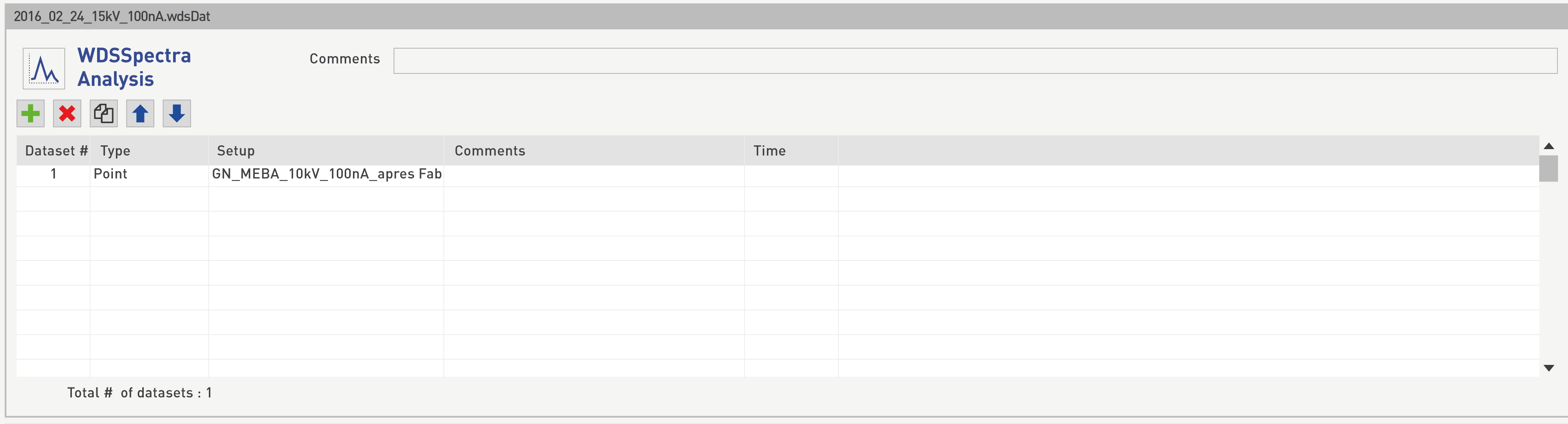
A last and useful information is provided at the bottom of that sub-panel as the the total number of datasets is given, along with the expected Total Time expected for the full analysis.

Images & Profiles Analysis

In order to create an Analysis file in the Images & Profiles mode, users have to select the ‘Images & Profiles’ icon with the ‘Analysis’ mode enabled. One can either use the File  New  Analysis  Images & Profiles string or directly edit the properties of the panels below the icon menu. User can also click on the ‘Acquire Now’ button available through the WDS Spectra Setting panel.

Any WDS Analysis file will be easily recognized by its « .impDat » extension. Therefore, once defined, this name will also be associated to the Properties and the Images & Profiles Analysis panels.

The general window layout of this menu is exactly the same as for the layout detailed for the WDS Spectra Analysis menu, with specific additions within the DataSet # and DataSet # Options sub-panels, since information have to be given with respect to the imaging aspect of that mode. Therefore, users should refer to the WDS Spectra section in this chapter for DataSet # creation, similar DataSet # Options and Common Options features already discussed in that section.

In this section we will focus on the options that are specific to the Images & Profiles Analysis mode.

The first step in the definition of an Images & Profiles Analysis file would be to assign a specific stored « .impSet » file to a specific location. The folder icon allows users to choose from a list of « .impSet » files (see the WDS Spectra section in this chapter for details).

The second part of the DataSet # definition has to be sub-divided into small sections as eight choices are possible for the ‘Data Type’ options, as a matrix of Profile, Image, Polygon and Mosaic applied to Beam or Stage modes. These choices will be detailed below.

Profile by Beam motion

The Profile by Beam Motion option described below allows the acquisition of a line profile by beam motion. X-ray signals can be acquired simultaneously with video signals.

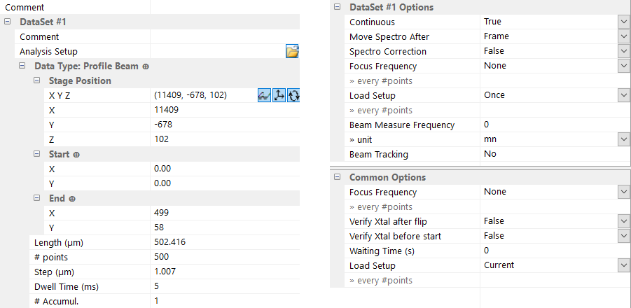
Close to the ‘Start’ and ‘End’ stage positions in the ‘Data Type’ sub-panel, the ‘+’ icon enables the selection of the line that is superimposed to the real-time monitor. After the line size and orientation are correctly set, users can click on ‘Done’ to validate their choices.

‘Start’ and ‘End’ line position values are indicated in µm but note that the size of the image should not exceed 50 µm in X or Y to avoid spectrometer defocusing.

Since each DataSet # is treated as an individual entity, it is recommended to Save the « .impDat » file along its building process.

The same explanations provided for the ‘WDS Analysis’ sequence can be applied to the ‘Images & Beam Profiles Analysis’ section of this chapter.

Profile by Stage Motion

The Profile by Stage Motion option described bellow defines the acquisition of a line profile by stage motion.

The X, Y and Z positions have to be given as ‘Start’ and ‘End’ values.

Image by Stage Motion

The Image by Stage Motion option described below rules the acquisition of an image by stage motion using either the [Center Stage] or the [3 Corners] configuration as ‘Definition Mode’. X-ray signals can be acquired simultaneously with video signals.

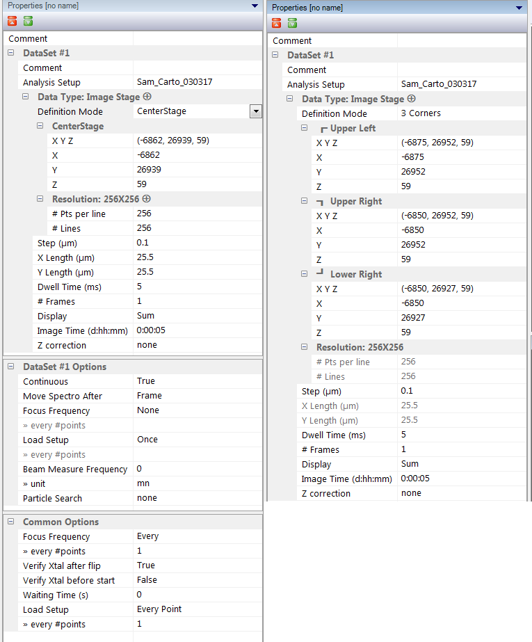
The image size and resolution are hence calculated once the three corners are set or when center and dimension are properly typed. With the stage increment being defined, an algorithm automatically computes the number of pixels per line and per frame. This feature is only available for images acquired by Stage Motion.

As images can cover wide surfaces, a Z-focus update could be needed to ensure a perfect focus on each pixel of the image. To do that, the Z correction option is applied for the DataSet# definition of both Center Stage and 3 Corners options. The Focus frequency can also be set under the Common Options panel.

The Center Stage option is often used to acquire an image on a flat but tilted surface. The Z value will be linearly adjusted during the acquisition through the ‘Z correction’ option under the ‘Resolution’ sub-panel, according to the Z values pre-recorded at the four corners of the stage.

Image by Beam Motion

Users can acquire an Image by Beam Motion as illustrated below using the Center Stage option.

Particle Search option is discussed in the SX-Results section.

The ‘Video Capture’ option can be enabled to define the acquisition of an image (BSE or SE or ABS or X-Ray) by capturing the whole image instead of a pixel-by-pixel acquisition. This acquisition mode is faster than the pixel-by-pixel acquisition.

Mosaic by Stage Motion

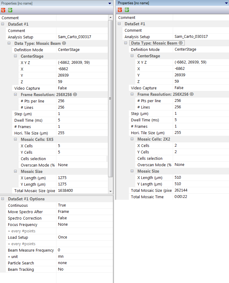
The fifth option presented to acquire Images and Profiles is called the Mosaic by Stage Motion and can be achieved by using a Center Stage position or a 3 Corners options similarly to the Image by Stage Motion case.

This mosaic mode corresponds to the collection of series of single X-Ray maps (cells or tiles) acquired by stage motion repeated over large areas. After the first cell acquisition, the stage is moved to the next cell and acquires it by stage motion. This pattern repeats until the last tile of the mosaic where the entire image can be reconstructed into the SX-Results program.

If the Center Stage mode is enabled, it coincides with the center of the mosaic. For a setup according to the 3 Corners option, please refer to the explanations given for ‘Image by Stage Motion’ above.

The total mosaic size computed is a function of the number of automatically or manually selected cells within the ‘Cell Selection’ utility.

Note: The mosaic mode is very sensitive to the image rotation. Indeed, as the stage moves in X and in Y between 2 consecutive frames, if the rotation is not properly adjusted, there will be a mismatch in the reconstruction. It is therefore useful to keep a noticeable feature on the same horizontal line.
Tip: If a tungsten filament crash down during the mosaic acquisition, the later can be restart from de last acquired cell.

In order to further minimize the mismatch between frames, it is possible to enable the Overscan function in the Mosaic Cells sub-panel, such that the rastered area is slightly larger than the initial computed tiled area.

In SX-Results program, the Overscan will be corrected with the function Results Processing/ Image Overlap Correction.

When a very long acquisition is performed, a beam intensity drift is expected and may induce some errors in the measurements. Therefore, by enabling the ‘Beam Measure Frequency’ functionality found under DataSet # Options sub-panel, the beam intensity will be recorded periodically in a pre-defined time interval in minutes. The intensity variation will automatically be stored in a file « filename_BeamMeas.txt » that monitor the ⁰/₀₀₀ beam current variations. The later file is stored in the current Project name/Sample Name/ Image and Profiles folder.

If a beam drift occurs, the image file can be corrected with the Beam Current Correction in Results Processing.

Mosaic by Beam Motion

The Mosaic by Beam Motion shares the two definition modes of Center Stage and 3 Corners with the Mosaic by Stage Motion. It corresponds as well to the acquisition of series of single X ray maps (cells or tiles) acquired this time by beam motion repeated over large areas. After the first cell acquisition, the stage is moved to the next cell and acquires it by Beam Motion, this pattern being repeated until the end of the mosaic where the entire image can be reconstructed into the SX-Results program.

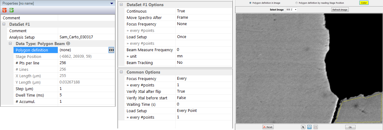
Polygon Beam

Another way to define the image area is to select a polygon. When the polygon mode is selected, a dedicated window automatically opens to define the size and the shape of the polygon. The two methods available to define the shape of a polygon are the Polygon by Stage and the Polygon by Beam. An example of DataSet # Option is provided below for the Polygon by Beam.

Beam scanning is restricted for areas that are below 100 µm in width.

In order to use this mode properly, users would have to select the sample area to analyze and the video image parameters on the real-time monitor. The Refresh Image would be activated when the image quality is satisfactory. At that point, a Polygon could be defined within the displayed image by drawing it vertex by vertex using a series of left clicks.

One should first select the sample area to be analyzed and the video image parameters on the real time screen. When the video image is well defined, click on the “Refresh Image” button. Once the Polygon is closed by superimposing start and end points, validation of this shape is done by clicking on the ‘OK’ button.

Polygon Stage

When choosing the [Polygon Stage] option, it is first required to select the sample area to be analyzed and the video image parameters on the real time monitor. The Polygon to draw has to be defined by moving the sample stage to each vertex of the desired figure and successively record each vertex by clicking on the Read Stage Position (glasses) icon, as shown Below.

Calibrate Analysis

The ‘Analysis’ mode button together with the ‘Calibrate’ icon allow one to create, modify or save the Calibrate Analysis file. The File  New  Analysis  Calibrate string allows also to create that type of file, which will affected by the « .calDat » extension.

The general window layout is simpler than for the ‘WDS Spectra’ and ‘Images and Profiles Analysis’ files: ‘Data Type’, ’DataSet Options’ and ‘Common Options’ panels on the left hand side face a table on the right hand side with the coordinates corresponding to each Point #.

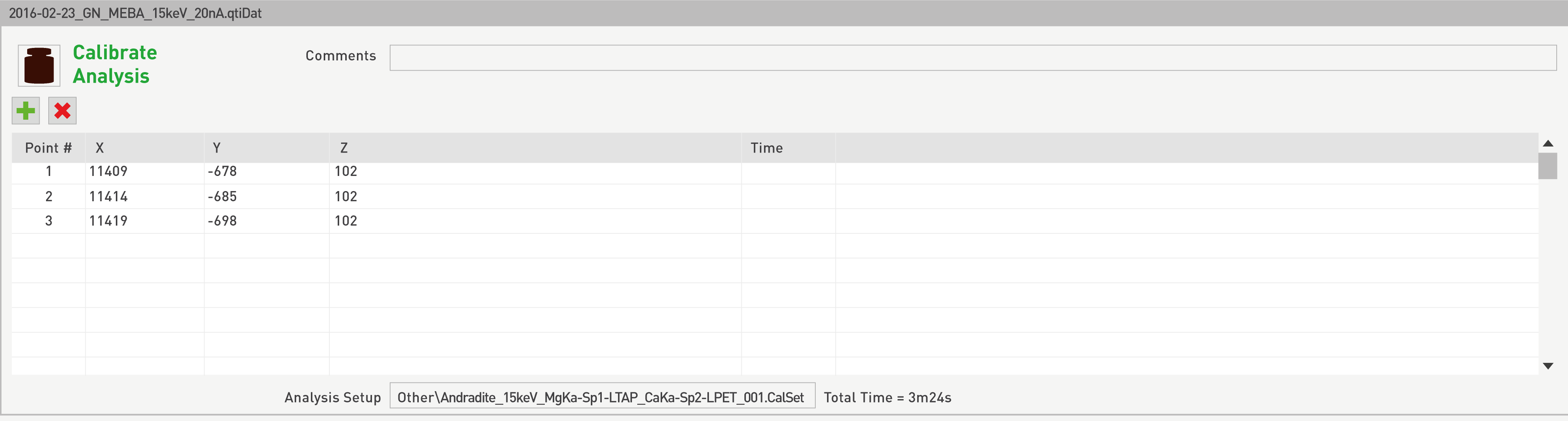
Prior to selecting locations to be calibrated, common settings under the Properties window such as ‘Method’ and ‘Auto-increment File name’ have to be set. Please refer to the ‘Calibrate Settings’ section for information about them.

In addition, the ‘Analysis Setup’ has to be chosen from an existing list of « .calSet » files.

Once a « .calSet » file is used as an ‘Analysis Setup’, users would apply this Setup to Points in X, Y and Z. 

Note: since samples might not be completely flat, it is recommended to proceed to a Z Auto-focus step using the ‘Focus Frequency function’. If the points are closely spaced, the Z Auto-focus could be done Once. Otherwise, for points located far apart from each other, one could order the Z Auto-focus to be done at Every Point.

Since other measurements could have been performed on a spectrometer of interest but using a different crystal, having the ‘Verify Xtal’ after flip option means that the system will automatically check and adjust the mechanical position of the crystal with respect to a pre-defined standard location. For maximum confidence in the analysis, some users may activate the ‘Verify Xtal’ before start, even when there is no crystal rotation involved prior to launch the Calibrate Analysis.

For certain samples, setting the ‘Background Measurement’ function to [Once] could be sufficient, whether throughput is a matter of interest, or beam sensitivity with respect to an element of interest is a concern. If this function is set to [Every], then the background will be measured on every single analysis point and may provide better statistical analysis.

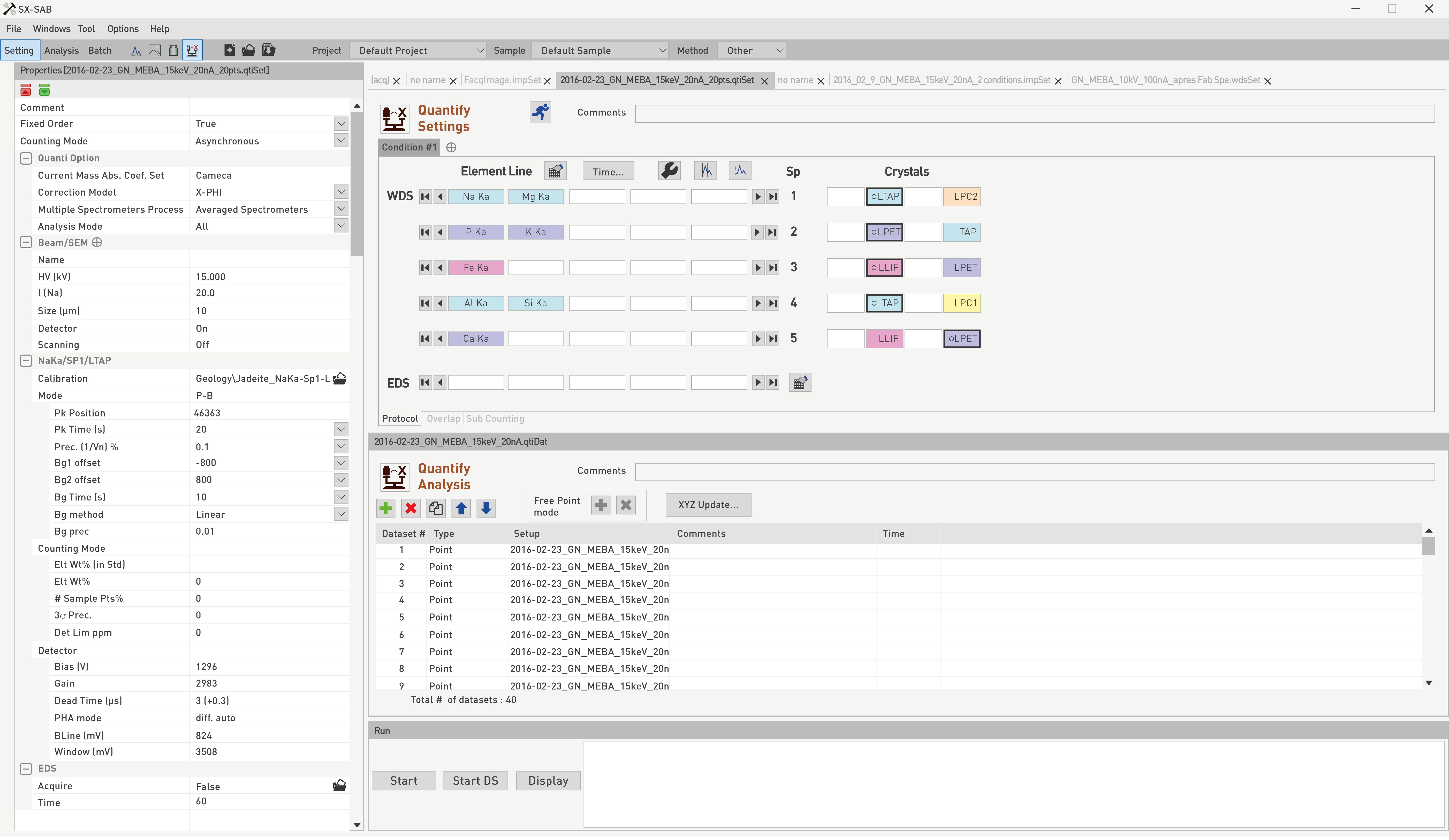
Quantify Analysis

The analysis menu will focus on the sample quantification, by using the ‘Analysis’ mode button combined with the ‘Quantification’ icon. A quantification file with the « .qtiDat » extension can also be created when following the File  New  Analysis  Quanti string. 

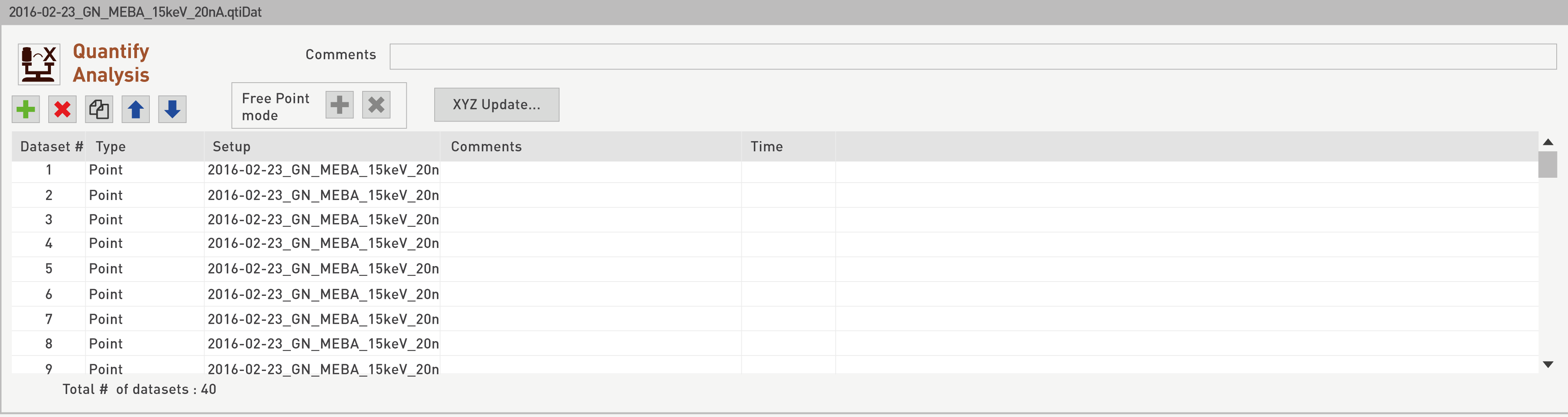
The general window layout is made of DataSet #, DataSet Option and Common Options windows while a table will be displayed on the right hand side with the coordinates corresponding to type of each DataSet.

The DataSet # creation links a Quantify Settings file (« .qtiSet ») with a Data Type, which will translate into a total analysis Time. Within the ‘Quantify Analysis’ file organization, users may consider preparing several Data Types such as Points, Lines or Grids, based on Stage or Beam motions.

For any of the Data Type selected, the Dataset # and Common Options will be the same as shown above, with the exception of the ‘Beam Tracking’ option, only available whenever the ‘Beam position’ is of interest in the definition of the DataSet.

Please refer to the ‘Calibrate Analysis’ section in this chapter for explanations, especially for options pertaining to the proper positioning of the crystals with respect to the spectrometers (‘Verify Xtal’), the measurement of the background (‘Background Meas. Frequency’), the ‘Focus Frequency’ and the selection of a beam setup (‘Load Setup’).

Data Type: Point

Individual analysis locations can be targeted and associated to a Quantify Settings file by selecting the Data Type: [Point] mode. The X, Y and Z coordinates are either typed, or automatically read by physically moving to a stage position and clicking on the ‘glasses’ icon. Once the DataSet is saved, double-clicking on it will drive the stage to the recorded location. There is no limit on the number of Points that users could define and store. Moreover, different ‘Quantify Settings’ files could be applied to several Points within the same DataSet.

Common to all the Data Type listed choices, the Quantify Analysis panel, located on the right hand side of the main quantification window, possesses five main icons. They are designed to help users organize very quickly and efficiently a DataSet, which can be created, deleted, duplicated, moved up or down a priority running list using dedicated icons above the DataSet table.

Data Type: Line Beam

Users can define a [Line Beam] Data Type, consisting in entering (X, Y) values for a starting point and an ending point for the beam. The ‘Length’ is automatically generated, as well as the ‘Step (µm)’ based on the total ‘#points’ chosen by analysts.

Note: the Stage Position records all three X, Y and Z coordinates but the beam positions, either at ‘Start’ or ‘End’, do not have the Z focus position recorded.

DataSet # Options and  Common Options panels could help in defining for instance a Focus Frequency and ensure that the Z focus value is correct.

Data Type: Line Stage

An alternative to using the [Line Beam] Data Type consists in using rather the [Line Stage] Data Type. Indeed, this Stage option allows as well to define ‘Stage Start’ and ‘Stage End’ locations with all (X, Y, Z) values indicated, and by choosing the number of points for the analysis, the ‘Step (µm)’ value is automatically calculated based on the total ‘Length (µm)’ analyzed. The added value of the Line Stage option resides in the ‘Profile Option’ sub-menu that allows [Non Flat Line] and [Variable Steps] choices.

Non Flat Line

With the [Non Flat Line] option, a quantitative line profile with variable Z coordinates can be envisioned. This functionality is particularly helpful when warped specimens have to be probed. The curvature is defined by selecting a number of points for which the Z coordinate is updated, and the curvature fitted by linear interpolation between adjacent points.

Variable steps

If several features have to be probed along the same line profile, then users may find some advantages into using non-equidistant steps. Users can set Length, Intervals and Step values for each segment belonging to the Line Stage. The Adjust button for each Segment compensates for any uneven calculation and brings the total % of covered length to 100%. A maximum of 5 segments can be defined.

Instead of defining individual [Points] or [Lines] as ‘Data Type’, users may define an array of points contained in a matrix using the [Grid Beam] mode as shown below. By default, three ‘Grid sizes’ come as square matrices of [10x10], [20x20] or [30x30] ‘#Pts per line’ by the equivalent ‘#Lines’. However, users may alter these default values by selecting a suited ‘# Pts per line’ by a desired ‘#Lines’ without any constraint and these choices will be reflected in the analysis sequence. The Center Stage or central point of the Grid has to be indicated by clicking on the glasses icon. Depending on the X and Y ‘Lengths (µm)’ and the ‘Total #pts’ values, a ‘Step (µm)’ will automatically be computed.

Data Type: Grid Stage

Analogous to the differences between [Line Beam] and [Line Stage] ‘Data Types’, the [Grid Stage] ‘Data Type’ allows users to be more flexible than the [Grid Beam] option by offering either a central point from where an array will be defined or by positioning the stage using three out of the four corners. Moreover, in the [Grid Stage] mode, the Z correction option applied for Non-Flat samples will be available, and will work exactly as described in the Line Stage section of this chapter. R

Data Type: Free Pts

The [Free Pts] ‘Data Type’ mode shown below is only available when used in conjunction with the ‘Stage Motion’, and permits the allocation of multiple points within a single DataSet without the need to define these points as part of a Line or a Grid.

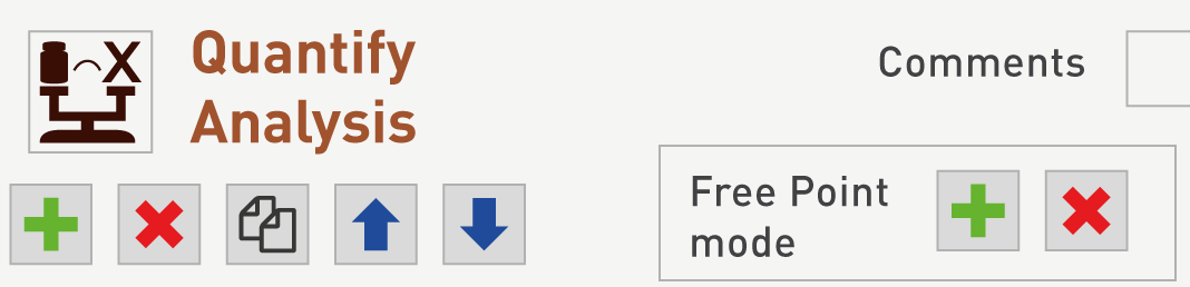
When this ‘Data Type’ is selected, a frame dedicated to add or remove points is enabled within the ‘Quantify Analysis’. 

Whether users consider building DataSets using a grid or a line ‘Data Type’, there is always a possibility to apply the ‘Quantify Analysis’ setup to individual points by selecting the Convert to Free Points option available in the ‘Data Type’ list.