SX-SAB – Setting

Overview

The first main function of the SX-SAB is the ability to create or modify all the hardware and software settings that will rule data acquisition. WDS Spectra, Images & Profiles, Calibrate and Quantification are described below. A tutorial section (link) is available to guide users on defining proper settings and options as applied to specific cases.

WDS Spectra Settings

In order to create a Settings file in the WDS scan mode, users have to select the WDS Spectra icon within the ‘Setting’ mode highlighted. One can either use the File  New Settings  WDS Spectra string or directly edit the properties of the panels below the icon menu.

By default, as an initial window organization, on the left hand side, a Properties panel with the chosen name for the file will display various parameters such Beam/SEM, Spectrometer # and Crystal type, and EDS. On the right hand side, a WDS Spectra Settings panel is made available to select a specific crystal for each individual spectrometer as well as the scanning range to be applied.

Any WDS Spectra settings file will be easily recognized by its « .wdsSet » extension. Therefore, once defined, this name will also be associated to the Properties and the WDS Spectra Settings panels.

The Beam/SEM conditions can be named and saved with all the associated parameters such as the accelerating voltage HV (kV), the beam current I (nA), the beam Size (µm), as well as Detector and Scanning states. In addition, by clicking on the ‘+’ icon, a sub-menu becomes available to enable a rapid setup of the Beam/SEM conditions.

With the Flash options, one could directly apply the current Beam/SEM conditions to this Properties panel, while the Select options will fetch previously stored conditions that could then be loaded, read, and finally applied by clicking on the dedicated icon.

Although WDS systems are ideal to analyze trace elements in a serial scanning fashion, it is sometimes useful to take advantage of the integrated EDS system (optional) operating in a parallel scanning fashion to probe major elements in a material. This EDS scan is enabled or disabled by selecting True or False respectively, along with a scanning time in seconds.

For each spectrometer, users are invited to define ‘Crystals’, ‘Range’ types and ‘Start/End’ values for the spectrum scan. The scan can be achieved with one or more spectrometer according to the studied chemical elements.

For information on the Detector parameters, please refer to the SX-Control section.

If the ‘Full Range’ option is selected for a chosen spectrometer and crystal pair, then the WDS scan will occur on the entire spectrometer range. 

However, one might select a central X-ray line position and request a ‘Relative’ scan from this line by typing in a scan width on either side. Note that the scan width does not have to be similar on both sides.

A third scanning option would consist in entering an ‘Absolute’ scanning range that the WDS would operate, irrespective of an X-ray line. Similarly, to the Beam/SEM conditions, the currently applied spectrometer and crystal scanning conditions could be readily imported into the Properties panel by using the Flash icons.

SxSAB Images and Profiles Settings

In order to create a Settings file in the Images and Profiles mode, users have to select the ‘Images & Profiles’ icon within the ‘Setting’ mode highlighted. One can either use the File New Settings Images & Profiles string or directly edit the properties of the panels below the icon menu.

All ‘Images & Profiles Settings’ files will be saved with the « .impSet extension ».

Default window will display on the left hand side, a ‘Properties’ panel with the chosen name for the file where several parameters such as Beam/SEM, X-ray line, Spectrometer # and Crystal type, and EDS are listed. These parameters are defined as part of a ‘Condition’. On the right hand side, an ‘Images & Profiles Settings’ panel allows the selection of a specific X-ray line, background offset, crystal type for each spectrometer as well as the detector type used in the SEM, as illustrated below.

Similar parameters defined in the WDS Settings menu will apply to the Images & Profiles Settings menu, with an additional level of precision consisting in focusing on specific elements through the selection of X-ray lines instead of defining ranges with respect to a spectrometer.

For a given set of accelerating voltage and beam current, known elements can be directly selected with their appropriate X-ray lines using the periodic table icon. The glasses icon will impose imaging and line profiling at a current X-ray line value set for the spectrometers within the SX-Control Panel .

Each defined Condition can only accept one X-ray line per spectrometer and crystal at a time. If more than one element is to be probed by the same spectrometer and crystal pair, then up to four Conditions can be defined by clicking on the ‘+’ icon close to the ‘Condition’ tabs.

The value typed in the ‘Bg Offset’ window will provide the shifted position with respect to the X-ray line of interest. Recorded ‘Images & Profiles’ will therefore highlight the presence and distribution of the elements of interest defined in the Settings files. In order to clearly highlight a difference between a selected peak and the background contribution, it is common practice to acquire data off-peak. 

SxSAB Calibrate Settings

Standardization or calibration steps start with the definition of ‘Calibrate Settings’ files as illustrated below and accessed by the combination of the ‘Setting’ mode and ‘Calibration’ icon.

All Calibrate Settings files will be saved with the « .calSet extension. »

Under the ‘Properties’ panel, beside the Beam/SEM parameters and the X-ray line associated to the Spectrometer and Crystal pair, users are given the options to allocate their calibrations to a Method based on their main interest. Some EPMA users might be focused on Geology, some on Metallurgy and others interested in the detection of Sulphides. Users who do not fall into these three categories could always elect an unclassified Method as ‘Other’.

 C:\Cameca SX Shared\Calibrations\Data\ 

Since calibrations ought to be performed on a regular basis, overtime users could choose to keep the same name for recurrent ‘Settings’ files, but differentiate them by applying the Auto-increment File name option.

Under the ‘Calibrate Settings’ icon, alongside the WDS parameters to be filled, the displayed icons fulfill the following functions:

- The top periodic table defines a standard specimen used for the calibration. One  element can be selected on each available spectrometer. 

- The periodic table dedicated to each Spectrometer/Crystal pair, defines the elements of interest for calibration, by electing an X-ray line (peak) compatible with the beam conditions. Only one element can be declared per spectrometer. 

- The spectrum icon allows users to choose the background limits around a selected peak. Initial limits are given by default, and can be changed upon a WDS scan triggered by the ‘Acquire Now’ icon.

- The most suitable conditions can be directly transferred to the Properties panel by clicking on the glasses icon.

Calibrations have to be as complete and detailed as possible in order to englobe all the potential roadblocks or obstacles faced during the normal acquisition state. To ensure a high confidence level, calibrations need better statistics than those commonly accepted during a regular acquisition. The signal to noise ratio, also defined here as Peak (P) to Background (B) level has to be well characterized and that is the reason why the Properties sub-panel in the Calibrate Settings files have to include an additional section on P and B, as compared to the WDS and Images & Profiles sections.

For this ‘Calibrate Settings’ section, we will therefore focus on the definition of Peak and Background methods, along with the Precision levels that could be achieved.

P-B Mode

The P-B mode is the most widely used for the ‘Calibrate Settings’. The maximum intensity is recorded at the top of the peak defined by the X-ray line and the background level is measured outside the peak.

Users have to type a ‘Pk (Peak) Time (s)’ and the background offsets (‘Bg 1’ and ‘Bg 2’). Althrough predefined values are available for immediate selection, any value could be typed in. Values for Bg1 Offset and Bg2 Offset are by default negative and positive respectively but it’s important to know that offsets can be both negative or both positive, depending upon the situation. For instance, the background could be curved, higher on one side with respect to the other side. Or there might be so many elements close to each other that choosing a background level on one of the side would be problematic and lead to erroneous results.

Note: if one of the background offsets has been set to None, then the background method option (Bg method) is replaced by a ‘Slope’ within the ‘Properties’ Panel. This technique is used to increase throughput for instance.

If a user decides to avoid recording any background at all by setting the Offset values to None, then a nominal value has to be set for the background in cps/nA.

In the Linear background calculation method, the background is estimated at the peak position with a linear extrapolation of measurements acquired before (left side) and after (right side) of the peak position.

As the background under the peak cannot be directly measured, it must be calculated using a Slope factor defined by drawing a linear extrapolation between both background measurements. The Slope factor is calculated as:

\[1+ \left( \frac{(P-S_1)}{(S_1-S_2)} \times \frac{(B_1-B_2)}{B_1} \right) \]

S1 and S2 are the first and second background positions in Sin θ unit.

B1 and B2 are the background intensities at positions S1 and S2.

P is the peak position in Sin(θ) unit, where the peak intensity is maximum. The net intensity peak I is calculated by subtracting the raw intensity peak P and the background intensity B.

In the Exponential background calculation method, the background is estimated at the peak position with an exponential extrapolation of measurements acquired before (left side) and after (right side) of the peak position. This method is especially well suited for X-ray lines measured on the PC-type crystals. (see Peak Area Mode below).

In order to obtain the background level under the peak, a few guidelines must be known:

- If the background increases as a function of the wavelength, the linear extrapolation is applied.

- If the background decreases as a function of the wavelength (most cases), then the applied formula is as follows:

\[I(B_g)=I(B_g+)\times \left(\frac{Pos(B_g+)}{Pos} \right)^f \]

With the exponent function f being expressed as:

\[ f=\frac{Log \left(\frac{I(B_g-)}{I(B_g+)} \right)}{Log \left(\frac{Pos(B_g+)}{Pos(B_g-)} \right)} \]

Where I(Bg) is the intensity under the peak, Pos is the position of the peak of interest in Sin(θ) unit, I(Bg+) and I(Bg-) are the intensities of the positive and negative background positions, Pos (Bg+) and Pos (Bg-) are respectively the positions of the positive and negative backgrounds in Sin(θ) unit.

Peak Area Mode

This mode can be used for the calibration of elements measured on the PC-type crystals when peak shifts and peak shapes differ between standards and unknowns. The measurement is based on the peak area and the user has to define the parameters of the area measurements.

When selecting ‘’Pk Area, users have to fill options dedicated to this mode such as the ‘# channels’ in the peak scan, the ‘Total Range’ which is the width of the peak in Sin θ unit, the background ranges (‘Bg range Left’ and ‘Bg range Right’) allowing the algorithm to determine a background shape, and finally a ‘Scan Time (s)’ representing the total counting time to scan the peak.

The Peak Time, ‘#channels’ and ‘Total Range’ are limited by the speed of the spectrometers. As a consequence, the parameters used for the acquisition can be slightly different than those used for the settings.

The speed of the spectrometers is the factor that restricts and controls the required parameters. The scan is performed in the continuous mode and as for any motor, there is a minimum speed. The Peak Time is the predominant factor and therefore, the number of channels and the time per channel are automatically computed based on the Peak Time value.

In the figure above, the blue curve corresponds to the acquired WDS scan, while the red segments (solid) delimit the background ranges and the blue curve (dash) represents the background fit. Under this configuration, the effective (net) peak area is contained by the area above the blue curve, while the area below it is considered as background.

SxSAB Quantify Settings

The Quantify Settings files are the last ones being created as they rely on results from WDS, Images and Profiles and Calibrate Settings in terms of the analytical parameters to enter.

All Quantify Settings files, which are saved with the « .qtiSet » extension, possess an extensive list of options or factors that deserve to be discussed prior to entering numerical values or in order to select the proper choice.

 

 

For all elements analyzed, the initial data is the relative intensity k = Ix/Istd

where Ix is the net intensity in the unknown specimen and Istd is the net intensity in the standard specimen. Both Ix and Istd have to be measured in the exact same experimental conditions. From the relative intensity, the correction program calculates the so-called K-ratio and then the true concentration.

The Quantify Settings panel illustrated on the figure below, is visualized by using the combination of the ‘Settings’ mode and ‘Quantification’ icon.

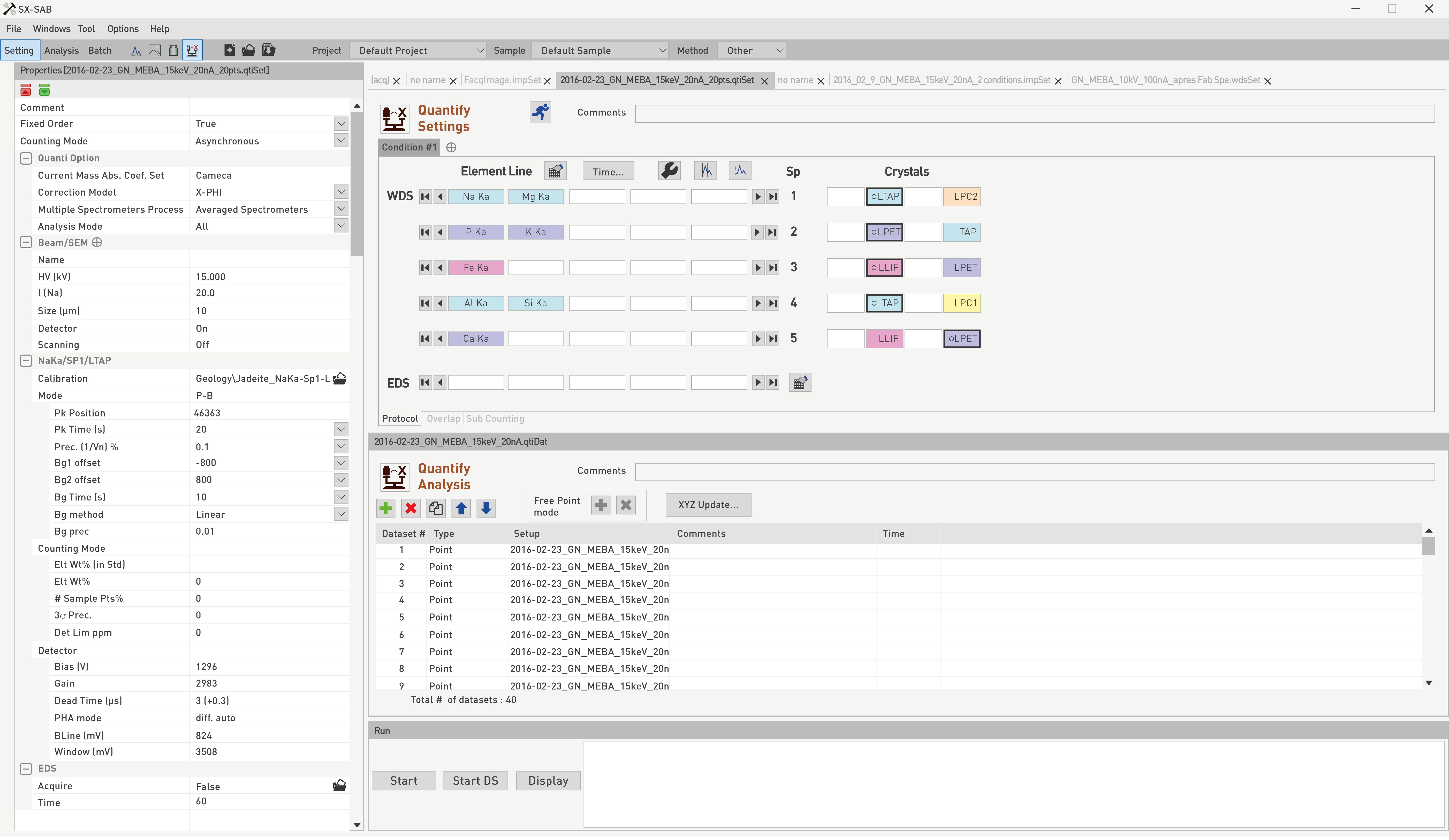
The first set of options to fill under the Properties sub-panel concerns Comment, Fixed Order and Counting Mode.

- Fixed Order: When several elements are measured on the same spectrometer (O Ka and B Ka on SP1/LPC2), if the ‘Fixed Order’ option is set to [False], the probe will start measuring O then B when probing the first point, B then O for the second point, and continue that alternated pattern as the analysis will progress for faster acquisition.

If the ‘Fixed Order’ is set to [True], then the order of appearance in the Settings file will prevail. In this case, O will always be measured first, and B afterwards. The order of appearance can be switched by dragging and dropping elements in the Element Line table using a left click.

- Counting Mode: When the Counting Mode is set to Asynchronous, a specific spectrometer will move to the next measurement as soon as the counting is achieved, even if the other spectrometers have not completed their counting sequence yet. This mode is preferred when throughput is a factor of interest.However, if users would like to avoid vibrations induced by the motion of the spectrometers, and especially while analyzing small particles, the Synchronous mode is to be elected. In this case, when a spectrometer has achieved its counting sequence, it will await the end of the counting sequence of the other spectrometers before moving to the next measurement. Therefore, there will be no spectrometer motion while another spectrometer is still counting.

Using the periodic table icon, users can select elements of interest which will be assigned to a spectrometer/crystal pair, based on the stored calibration files.

Since some spectrometers could contain the same crystal types, one could choose to proceed to the counting sequence on a different spectrometer/crystal pair than the location initially assigned, or to choose one spectrometer/crystal pair instead of several pairs.

In order to optimize the use of all the spectrometers, it is possible to set one element on several spectrometers and/or in several conditions. The measurements obtained for the multi-counted element are combined to calculate the concentration, the detection limit and the statistical precision. This mode is dedicated for the quantification of a trace or low concentration element to improve its counting statistics. The multi-counted element can be present on several spectrometers/conditions by using the “Duplicate” function which is accessible through a right-click on each element on the ‘Quantification Settings’ panel:

The following figure will detail the Quanti Option section found under the Properties sub-panel of the Quantify Settings file.

- Current Mass Abs. Coef. Set: By default, the Mass Absorption Coefficient Set (MAC Set) is the CAMECA built-in version. Users interested in different calculations could choose another method located in the ‘MAC Set’ program part of the SX-Utilities .

- Correction Model: The two correction models available are the X-PHI and the PAP, as discussed at the beginning of this section.

- Multiple Spectrometers Process: For statistical reasons, users could decide to measure specific elemental X-ray lines on several spectrometers, and to proceed to an averaged calculation or to a summed calculation. The latter is more often used when count numbers are low, and a summation is required to increase the ability to quantify these trace amounts.

Time optimization

A good appreciation of the throughput is given per element and per spectrometer by clicking on the ‘Time…’ button as shown on general figure above.

This function allows to check rapidly the peak and background measurement timing events (e.g., for O and B on the same spectrometer) by positioning the mouse on a measuring segment. Dragging lines defining a segment will modify its duration. ‘The Time…’ button changes into the ‘Elts…’ button. Both sub-panels are inter-changed by toggling between these two buttons.

In case a lower (Bg-) and upper (Bg+) background measurements are scheduled, changes in the timing events will apply to both simultaneously. For statistical reasons, keeping a defined ratio between peak and background counting times might be needed, and can be achieved by dragging a segment line with a left click in conjunction with the CTRL keypad.

Background selection

This function allow user to select the positive and negative background regarding geometry of simulated or measured peak. Measured spectrum can be import from «.wdsdat» files. Vertical lines that identify background position can be draged by clicking on. 

Spectrum simulation

This function allows users to simulate WDS spectrum from the selected chemical elements. Results are displayed through the SX-Results program and can be treat as any WDS spectrum (see SX-Results chapter for more informations). User has to enter the Elt wt% before running the spectrum simulation.

Config optimization

When all the analytical parameters are defined, the optimizer button can be used to finely improve the setting file. When actions are done, a pop-up windows appear and indicate the end of the automated task.

Analysis Modes

Six Analysis Mode options are offered to the users based on their materials of interest and will be detailed below : All, By Stoichiometry, By Difference, Oxide like (Stoichio and Diff), Matrix Definition, Matrix Definition and Stoichio.

[All] mode 

All the elements pre-defined in the X-ray table will be measured. The overall contribution of all the measured elements should total 100%.

[By Stoichiometry] mode

For one element (oxygen in many cases), this element must not be present in the list of the elements declared in the X-Ray table. In the ‘Valence’ table, select the desired valence for each element. The most common valence is proposed as default value.

In some minerals, F and Cl for instance can be measured. Those elements have negative valences and cannot be calculated as an oxide form. Their valences will be forced at 0 in order to have their calculation done in wt% only.

The [GeoSpecies] calculation is a software option used by geologists or mineralogists who want to measure an unknown mineral based on a known structural formula.

The unknown specimen is still measured as in the [Stoichiometry] option (all cations are measured and the anion is calculated by stoichiometry).

The user has to select the specie (Apatite, Axinit, Carbonate etc.) and he can do some modifications by clicking on “Edit”. 

The quantitative results will be displayed in SX-Results window in wt. %, in at % (normalized to 100 % ) and in oxide %. For the applications dedicated to Geology the SX-Result window will also display a feature called ‘GeoQuant’ providing the number of cations normalized to a specified number of oxygens.

[By Difference] mode

It would allow users to quantify the presence of an element by difference to 100 wt.% with respect to the other elements. This is well-suited in the case of C for instance, as this element is not easy to analyze.

[Oxide like (Stoichio and Diff)] mode

One could take advantage of both the Stoichiometry and the Difference modes by using the [Oxide Like] option. One element is calculated by stoichiometry while a second element is obtained by the remaining amount to reach 100 wt.%. The Definition of the Oxide-Like type includes the cations selection, the element calculated by difference, its anion and all their respective valence numbers. In almost all cases the cation measured by difference is Hydrogen with a valence of 1 and the anion is Oxygen with a valence of -2. This mode is mostly used by Geologist to analyze minerals containing H₂O.

[Matrix Definition] Mode

The figure below indicates that the [Matrix Definition] option is active with minor elements compared to the main matrix of elements constituting the material of interest. The matrix composition has already been entered and could be as close to 100 wt.% as one wishes. In other words, there is no minimum threshold required for the trace elements entered.

[Matrix Definition and the Stoichiometry] mode

It enables users to add to the initial matrix an element with fixed concentration (Set Matrix) while oxygen is calculated by stoichiometry for all the elements considered.

Users can refer to the WDS settings section for the Beam/SEM parameters as they are identical in the Quantify Settings section.  A probe size of zero µm indicates that the beam is tightly focused, and therefore any other values (positive) imply a defocusing of the electron beam on the specimen.

Quantify Settings files

In the ‘Quantify Settings’ files, the Element/Spectrometer/Crystal window will display exactly the same parameters illustrated in the following figure, with a few additions that are described below such as the Calibration option and the Expected Statistics:

‘Quantify Settings’ files need to be paired to ‘Calibration’ files where parameters for the elements of interest would have been well established. In figure above for instance, the element F will be probed and all the calibration parameters such as spectrometer, crystal, Method, Beam Conditions, WDS conditions, Detector conditions and Background models are readily accessible through an ‘Open File’ icon. Users can drag and drop column header to sort data.

By default, when an element is defined, peak and background counting times are matched to those used during the standardization or calibration. Nevertheless, depending of the concentration to measure and the desired precision, one might to change the counting times coming from the calibration file. For high precision and low concentration detection, the counting times may be as long as several minutes in the most difficult cases.

Precision is expressed in %, as \[\frac{1}{\sqrt{1}} \] where is the accumulated number of counts.

The counting sequence will stop if the desired precision is reached before the set counting time. For example, with a large counting time and a requested precision of 0.5 %, the counting will stop when the accumulated counts will reach 40,000 counts. For a requested precision of 1%, the counting will stop when the accumulated counts will reach 10,000 counts.

Based on the number of points used for the acquisition, the ‘Expected Statistics’ will vary. So users can estimate how many points they should probe in order to reach a certain confidence level (3σ precision) or a minimum detection limit (ppm).

Overlap

Another well-known issue encountered in EPMA during Calibration and Quantification concerns the overlap between closely positioned peaks. In order to compensate for this issue into the analytical process, a special tab ‘Overlap’, leads to an additional menu under the Quantify Settings panel.

In the example taken above, a possible interference between Sn Lα and Fe Kβ needed to be acknowledged and accounted for. Therefore, based on the peak position of the initial Sn Lα measured line, a list of overlapping lines is automatically generated within a range of +/- 600 Sin θ  for standard crystals, and +/- 2000 Sin θ  for Pseudo-Crystals (PC). If the event that the interference to be accounted for is not part of the pre-loaded list of X-ray lines, one can define the desired line by using the ‘User’ Button.

A list of standards available in the instrument is provided to calibrate this interference. It is crucial that the selected standard material does not contain the measured element initially defined (Sn here).

Several interferences could be chosen within the same standard by clicking on ‘Add’.

By clicking on ‘Acquire’, all interferences which ‘Acq status’ is set to [Yes] in the Overlap list will be run. The system will measure the intensity emitted by the standard at the spectral position of the X-ray of interest (Measured Line). Counting time and background offset are defined in the current setup. This acquisition will be done similarly as a calibration acquisition in manual mode. The sample stage is automatically moved to the standard position and an acquisition window will automatically open. This interference calibration will have the « .ovl » extension and will be stored in SXPC\Analysis Setups\Quanti\Overlap.

The stored file is dedicated to a given quantitative setup but it can be associated to other setups provided the analyzed X-ray lines are compatible with the lines involved in the overlap correction).

When the interference calibration acquisition is complete, the reference intensity is displayed in cps/nA in the ‘Overlap’ sub-panel, but this value could be manually modified.

When an overlap file is defined and associated to a setup, the calibrated interferences will be automatically corrected in the quanti result files.

The intensity of the overlapping lines measured during the setup definition, is corrected with respect to the matrix effect of the standards, using the X-Phi procedure. During the quantification procedure, the concentration off the unknown sample is calculated in first approximation with the interference. The final interference intensity is suppressed from the overlapped line.

Sub Counting

Various counting configurations can be explored in order to extract information in a more useful way based on materials, trace elements, sensitivity to electron beam, and background shape among few parameters.

Designing counting time patterns can be achieved using the ‘Sub Counting’ tab located at the bottom of the ‘Quantify Settings’ panel.

A list of seven choices is provided to the users and will be explained hereafter.

Sub-counting P,B,P,B…

Peak and background counting times of the selected elements are divided by the ‘Sub counting number’ n.  The sequence alternates peak and background sub-counting until the total value of the defined peak and background times has elapsed. The peak and the background intensities are the sum of the intensities measured during the n sub-counting sequence.

Sub-counting P,P,…,B,B…

Peak and background counting times of the selected elements are divided by the ‘Sub counting number’ n. The sequence measures n sub-counting on the peak followed by n sub-counting on the background until the total defined peak and background times are elapsed. Peak and background intensities are the sum of the intensities measured during the n sub-counting.

Time 0 Intercept

Only peak counting of the first defined selected elements are divided by the ‘Sub counting number’ n. The decay of the selected elements is plotted versus time and computerized to calculate the intensity at t=0. It is important to notice that the sequence of measurement will be automatically set to ‘Fixed Order’. This mode is especially suited for beam sensitive elements such as Na for instance. In this case, Na would be the first element analyzed to avoid degrading the measurement.

Decontamination AutoTest

A special attention is brought to beam induced carbon contamination. Therefore, the C peak counting time is divided by the ‘Sub counting number’ n. If the n results fulfill the Chi test, the measurement is kept and the next point will be analyzed. If the n measurements do not fulfill the Chi test, the first measurement among the n measurements is rejected and an additional measurement is repeated at the same point. The rejection of the first point among the n measurements will continue until the n measurements fulfill the Chi test with a ‘Maximum number of series’ m.

Chi² test

Peak counting times of the selected elements are divided by the ‘Sub counting number’ n. If the n results fulfill the Chi test, the measurement is kept and the next point will be analyzed. If the n measurements do not fulfill the Chi test, the n measurements are rejected and repeated at the same point. The n measurements will be repeated at the same point up to the ‘Maximum number of series’ m until n fulfills the Chi test. If after m series, the n measurements do not fulfill the Chi test, this point will be totally rejected and the next point will be analyzed.

Sub-Counting / Chi² P, B, P, B…

Peak and background counting times of the selected elements are divided by the ‘Sub counting number’ n. The sequence alternates peak and background sub-counting and a Chi test is automatically performed on all sub-counting measurement. If the number of measurements rejected after the Chi test is smaller than the ‘Max nb of rejected measurements’ m, the measurement is computed with valid measurements without any additional message in the SX Results. 

If the number of measurements rejected after the Chi test is larger than the ‘Maximum nb of rejected measurements’ m, the point is computed with all measurements in SX-Results.  This point will appear in bold font and an error message will be displayed as ‘Counting problem occurred on this point’. All measurements are visible into ‘Sub Counting’ window in the SX-Results program.

Sub-Counting / Chi² P, P… B, B…

Peak and background counting times of the selected elements are divided by the ‘Sub counting number’ n. The sequence measures n sub-counting on the peak followed by n sub-counting on the background a Chi test is automatically performed on all sub-counting. If the number of measurements rejected after the Chi test is smaller than the ‘Max nb of rejected measurements’ m, the measurement is computed with valid measurements without any additional message in the SX-Results.

If the number of measurements rejected after the Chi test is larger than the ‘Maximum nb of rejected measurements’ m, the point is computed with all measurements in SX-Results.  This point will appear in bold font and an error message will be displayed as « Counting problem occurred on this point ». All measurements are visible into ‘Sub Counting’ window in the SX-Results program (link).